LECTURE: Measuring Parallel Performance

Overview

Teaching: 20 min
Exercises: 10 min

Questions

• What is performance and how is it measured?

• What is scalability?

• What is meant by strong and weak scaling?

Objectives

• Learning how to measure the performance of software.

• Understanding the difference between strong and weak scaling.

• Understanding the importance of load balance.

Parallel performance

Why do we run applications in parallel?

In the course etherpad, write down why you think running applications in parallel is useful.

In general, there are two advantages to running applications in parallel: (1) applications will run more quickly and we can get our solutions faster, and (2) we can solve larger, more complex problems.

In an ideal world, if we increase the number of cores we are using by a factor of 10, we should be able to either get the solution to our current problem 10 times faster, or to run a system 10 times bigger in the same amount of time as now.

Unfortunately, this is often not the case…

How to measure parallel performance?

Measuring parallel performance can help us to understand:

• whether our application is making the most of the cores assigned to it
• the factors that can improve or hinder performance
• how best to use the application and available HPC resources

But, how do we quantify performance when running in parallel? Consider a system with an execution time of T - this time will depend on the size/complexity N of the system and the number of processors/cores P being used to run this system. One way to measure performance could be to consider the speedup of the system compared with a run on a single processor:

Ideally, the speedup increases in a linear fashion, meaning that as you double the number of processors used, your speedup will also double. However, this is rarely the case.

Another metric to consider is the parallel efficiency E(N, P). This is a measure of how the speedup changes as the number of processors used is increased:

Given that, in general, S(N, P) < P, it follows that E(N, P) < 1.

Finally, it can be useful to estimate the efficiency of the parts of your code that run only in serial. The serial efficiency E(N) is measured by:

Strong vs. weak scaling

Scaling describes how the runtime of a parallel application changes as the number of processors is increased. Usually, there are two types of scaling of interest:

• strong scaling is obtained by increasing the number of processors P used for a problem of fixed size/complexity N. As the number of processors increases, the amount of work per processor should decrease.
• weak scaling is obtained by increasing both the number of processors and the system size/complexity, with both of these being increased at the same rate.

Ideally, for strong scaling, the runtime will keep decreasing in direct proportion to the growing number of processors used. For weak scaling, the ideal situation is for the runtime to remain constant as the system size, and number of processors used, are increased. In general, good strong scaling is more relevant for most scientific problems, but is also more difficult to achieve than weak scaling.

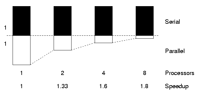
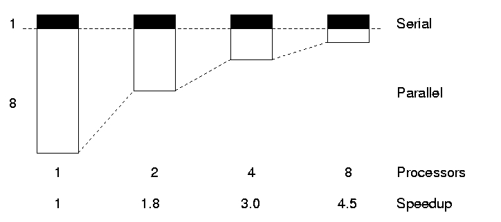
Amdhal’s law and strong scaling

The limitations of strong scaling are best illustrated by Amdhal’s law: “The performance improvement to be gained by parallelisation is limited by the proportion of the code which is serial”. As more processors are used, the runtime becomes more and more dominated by the serial portion of a code.

Analogy for Amdhal’s law

Consider a trip from Holyrood, Edinburgh to the Empire State building in New York. The distance from Edinburgh to New York is 5,200 km, and you can either fly with a Jumbo Jet (flight speed 700 km/hrs) or a Concorde (flight speed 2,100 km/hrs). What is the speedup of using the Concorde?

Solution

The Jumbo Jet will cover that distance in around 7h30, and the Concorde covers this in 2h00, so you might think that the speedup is 3.75x.

However, in this problem, we are not starting in a plane about to take off! There are additional times to take into consideration:

• Trip to Edinburgh airport: 30 mins
• Security and boarding: 1h30
• US immigrations: 1h00
• Taxi ride to downtown New York: 1h00

There is a fixed overhead of 4 hrs that we can’t reduce. When considering this 4-hour overhead, we find that our total trip by Jumbo Jet takes 11h30, whereas travelling by Concorde takes 6 hrs. Our speedup is therefore 1.92x not 3.75x.

Amdhal’s law suggests that, the shorter the journey, the more important the fixed (serial) overhead is in determining the total journey time.

Proof of Amdhal’s Law

Consider a typical program – this will have sections of code that could potentially run in parallel, and sections that are inherently serial and can’t run in parallel. Let’s further suppose that the serial code accounts for a fraction α of its runtime. If we can parallelise the potentially parallel part of the code with 100% efficience, then:

• the hypothetical runtime in parallel is:
• the hypothetical speedup is:

This means that speedup is fundamentally limited by the serial fraction. No matter how large P becomes, the speedup

Example for α = 0.1

• On 2 processors, the hypothetical speedup is S(N, P) = 1.8
• On 16 processors, the hypothetical speedup is S(N, P) = 6.4
• On 1024 processors, the hypothetical speedup is S(N, P) = 9.9

Gustafson’s law and weak scaling

Gustafson’s law provides a solution to the limitations of strong scaling described. The proposal is simply: we should run larger jobs on larger processor counts. If we run larger problems, then the parallelisable part of the problem will increase. We are still limited by the serial part of the code, but this becomes less important, and we can run on more processors more efficiently.

Analogy for Gustafson’s law

Let’s consider a new trip, one from Holyrood, Edinburgh to the Sydney Opera House in Sydney, Australia The distance from Edinburgh to Sydney is 16,800 km. As with our trip to New York, you can either fly with a Jumbo Jet (flight speed 700 km/hrs) or a Concorde (flight speed 2,100 km/hrs). Also, let’s assume that the overhead is similar to that for a trip to New York (so 4 hours). What is the speedup of using the Concorde this time?

Solution

The Jumbo Jet will cover that distance in around 24 hrs for a total trip time of 28 hrs, and the Concorde covers this distance in 8hrs for a total trip time of 12 hrs. The speedup is therefor 2.3x (as opposed to 1.9x for the trip to New York).

This is Gustafson’s law in effect! Bigger problems scale better. If we increase both distance (i.e. N) and maximum speed (i.e. P), we maintain the same balance of “serial” to “parallel”, and get a better speedup.

Proof of Gustafson’s Law

Let’s assume that the parallel contribution to runtime is proportional to the size of the system N. Then, the total runtime on P processors is: The total runtime on a single processor is: where α is the non-parallelisable fraction of the code. It follows that the speedup: If we scale the problem size with the number of processors (e.g. by setting N = P for weak scaling), then we expect a speedup S(P, P) = α + (1 - α)P , and an efficiency E(P, P) = α / P + (1 - α).

Load imbalance

The laws and thoughts above only apply to cases where all processors are equally busy. What happens if some processors run out of work while others are still busy?

Load imbalance in packing boxes

Consider fours people tasked with filling boxed with cans. Each of them is in charge of placing one specific type of can (so Anna is in charge of the chopped tomatoes, Paul is in charge of the chickpeas, David is in charge of the sweetcorn, and Helen is in charge of the spinach). It takes 1 minute for each person to grab one tin and place it in the box, and each person can only carry one tin at a time. Multiple people can place a tin in the box at the same time. How long would it take to fill this box?

Person	N. tins
Anna	6
Paul	1
David	3
Helen	2
Total	12

Solution

Because each task (each placement of a tin) takes 1 minute, the box will not be fully packed until Anna is finished. Therefore, it will take 6 minutes to complete this task.

In the event that the group could not move on to the next box until this box is fully packed, this would mean that Paul, David, and Helen would be doing nothing and waiting for Anna to finish for some time (5 minutes in Paul’s case!).

Scalibility isn’t everything! It’s also important to make the best use of all processors at hand before increasing the number of processors.

Quantifying load imbalance

We can define a “load imbalance factor” as being the ratio of the maximum load (the load on the most used processor) over the average load on all processors: LIF = maximum load / average load.

This is a measure of how much faster your calculation would be if your system was balanced. For a perfectly balanced system, LIF = 1.0, but this is rarely achieved. In general, LIF will be greater than 1.0.

For the box packing example above, the average load is 3 tins per worker, and the maximum load is 6 tins for Anna to pack. In this case, LIF = 2. We could therefore decrease the processing time by a factor of 2 by distributing the tasks more evenly!

Key Points

• As the number of cores are increased, performance rarely scales linearly.

• Scalibility changes as the size and complexity of the system is changed.

• Scalibility can be meaningless if the work load is not distributed evenly among processors.