Welcome
Overview
Teaching: 20 min
Exercises: 0 minQuestions
What can I expect from this course?
How will the course work and how will I get help?
How can I give feedback to improve the course?
Objectives
Understand how this course works, how I can get help and how I can give feedback.
Code of Conduct
To make this as good a learning experience as possible for everyone involved we require all participants to adhere to the ARCHER2 Code of Conduct.
Any form or behaviour to exclude, intimidate, or cause discomfort is a violation of the Code of Conduct. In order to foster a positive and professional learning environment we encourage the following kinds of behaviours throughout this course:
- Use welcoming and inclusive language
- Be respectful of different viewpoints and experiences
- Gracefully accept constructive criticism
- Focus on what is best for the course
- Show courtesy and respect towards other course participants
If you believe someone is violating the Code of Conduct, we ask that you report it to ARCHER2 Training Code of Conduct Committee by completing this form, who will take the appropriate action to address the situation.
Course structure and method
Rather than having separate lectures and practical sessions, this course is taught following The Carpentries methodology where we all work together through material learning key skills and information throughout the course. Typically, this follows the method of the instructor demonstrating and then the attendees doing along with the instructor.
Not a Carpentries lesson
Although we use the Carpentries style of teaching and the Carpentries lesson template, this is not a Carpentries lesson.
There are helpers available to assist you and to answer any questions you may have as we work through the material together. You should also feel free to ask questions of the instructor whenever you like. The instructor will also provide many opportunities to pause and ask questions.
We will also make use of a shared collaborative document - the etherpad. You will find a link to this collaborative document on the course page. We will use it for a number of different purposes, for example, it may be used during exercises and instructors and helpers may put useful information or links in the etherpad that help or expand on the material being taught. If you have useful information to share with the class then please do add it to the etherpad. At the end of the course, we take a copy of the information in the etherpad, remove any personally-identifiable information and post this on the course archive page so you should always be able to come back and find any information you found useful.
Feedback
Feedback is integral to how we approach training both during and after the course. In particular, we use informal and structured feedback activities during the course to ensure we tailor the pace and content appropriately for the attendees and feedback after the course to help us improve our training for the future.
You will be provided with the opportunity to provide feedback on the course after it has finished. We welcome all this feedback, both good and bad, as this information in key to allow us to continually improve the training we offer.
Key Points
We should all understand and follow the ARCHER2 Code of Conduct to ensure this course is conducted in the best teaching environment.
The course will be flexible to best meet the learning needs of the attendees.
Feedback is an essential part of our training to allow us to continue to improve and make sure the course is as useful as possible to attendees.
Understanding your HPC workflow
Overview
Teaching: 40 min
Exercises: 20 minQuestions
What are the components of my HPC research workflow?
What impact would performance improvements have on the different components?
How can I understand the dependencies between the different components?
Objectives
Gain a better understanding of my HPC research workflow.
Appreciate the potential impact of performance improvements in the HPC research workflow.
And what do you do?
Talk to your neighbour or add a few sentences to the etherpad describing the research area you work in and why you have come on this course.
In this section we will look at research workflows that involve an HPC component. It is useful to keep your own workflow in mind throughout. Some of the steps or components we describe may not be relevant to your own workflow and you may have additional steps or components but, hopefully, the general ideas will make sense and help you analyse your own workflow.
What do we mean by workflow here? In this case, we mean the individual components and steps you take from starting a piece of work to generating actual data that you can use to “do” research. As this is an HPC course, we are assuming that the use of HPC is an integral part of your workflow.
As an example, consider the following simple workflow to explore the effect of defects in a crystal structure (we know that this is simplified and does not contain all the steps that might be interesting):
- Step 1: Source crystal structure from experimental data or previous modelling studies
- Step 2: Convert crystal structure into input format for modelling using VASP
- Step 3: Define the input parameters for the planned calculations
- Step 4: Upload the input files for the VASP calculations to the HPC system
- Step 5: Run geometry relaxation on the input system
- Step 6: Analyse output to verify that relaxed (optimised) geometry is reasonable
- Step 7: Run calculations on relaxed structure to generate properties of interest
- Step 8: Download output from HPC system to local resource for analysis
- Step 9: Analyse output from calculations to generate meaningful results for research
Even this overly-simplified example has more steps than you might imagine and you can also see that some steps might be repeated as required during the actual use of this workflow. For example, you may need to try a variety of different input configurations for any of the calculations to obtain a reasonable model of the system of interest.
Your workflow
Talk to your neighbour (or rubber duck) and explain your research workflow. In particular, try to break it down into separate steps or components. Which of the components are the most time consuming and why? Why do the components have to be in the order you have described them?
What is worth optimising?
When thinking about your workflow, you should try and assess which components are the most time consuming - this may not be a single component, your workflow could have multiple components with similar lengths.
Is the use of HPC one of the most time consuming elements? If not, then improving the performance (or time taken) by the HPC component may not actually yield any improvement in the time taken for your workflow.
This situation is analogous to transatlantic flight (and to parallel performance on HPC systems, as we shall see later!). Transatlantic flight is essentially a very simple workflow:
- Step 1: Travel to the origin airport
- Step 2: Bag drop and navigate security control
- Step 3: Board aeroplane
- Step 4: Fly
- Step 5: Disembark aeroplane
- Step 6: Passport control and baggage reclaim
- Step 7: Leave airport and continue journey
For our example, consider that the “Fly” component is what we are looking at improving (say, by designing a faster aeroplane). At the moment, the components take the following times:
- Steps 1-3: 3 hours (1 hour travel to the airport, 2 hours to get onto the ‘plane)
- Step 4: 6 hours
- Steps 5-7: 1 hour
At the moment, flying represents 60% of the time for the total workflow. If we could design an aeroplane to reduce the flight time to 3 hours (let’s call this ‘plane, Concorde) then we could reduce the total time to 7 hours and flying would represent 43% of the time for the total workflow. Any further reductions in flying time would have less impact as the other workflow steps start to dominate.
Moving back to a research workflow involving HPC, if the HPC component of the workflow is a low percentage of the total time, then the motivation for optimising it (at least in terms of improving the overall workflow performance) is not very high.
Other motivations
Of course, improving the time taken for the overall workflow is not the only reason for optimising and/or understanding the performance of the HPC component. You may also want to maximise the amount of modelling/simulation you can get for the resources you have been allocated. Or, you may want to understand performance to be better able to plan your use of resources in the future.
Components and dependencies
As well as understanding the components that make up your workflow, you should also aim to understand the dependencies between the components. By dependencies, we mean how does progress with one component depend on the output or completion of another component. In the simplified workflow examples we have thought about previously, the different components were largely sequential - the previous component had to complete before the next component could be started. In reality, this is not often true: there may be later components that are not strictly dependent on completion of previous components. Or, our workflow may be made up of many copies of similar sequential workflows. (Or, even a combination of both of these options.)
When we do not have strict sequential dependencies between components of our workflows then there is the potential to make the workflow more efficient by allowing different components to overlap in time or run in parallel. For example, consider the following simplified materials modelling workflow:
- Step 1: Source crystal structures from experimental data or previous modelling studies
- Step 2: Convert crystal structures into input format for modelling using VASP
- Step 3: Define the input parameters for the planned calculations at a range of temperatures and pressures
- Step 4: Upload the input files for the VASP calculations to the HPC system
- Step 5: Run VASP calculations on HPC system
- Step 6: Download output from HPC system to local resource for analysis
- Step 7: Analyse output from individual VASP calculations
- Step 8: Combine multiple analyses/output to generate meaningful results for research
As there are now multiple experimental crystal structures to start from and multiple independent calculations at different physical conditions for each of the starting crystal structures we can rewrite the workflow in a way that exposes the dependencies and potential parallelism:
- For each crystal structure:
- (1) Source crystal structures from experimental data or previous modelling studies
- (2) Convert crystal structures into input format for modelling using VASP (depends on (1))
- For each physical condition set:
- (a) Define the input parameters for the planned calculations at a range of temperatures and pressures (depends on (2))
- (b) Upload the input files for the VASP calculations to the HPC system (depends on (a))
- (c) Run VASP calculations on HPC system (depends on (b))
- (d) Download output from HPC system to local resource for analysis (depends on (c))
- (e) Analyse output from individual VASP calculations (depends on (d))
- Combine multiple analyses/output to generate meaningful results for research (depends on completing all (e))
Assuming we have 5 different crystal structures and 10 different sets of physical conditions for each crystal structure we have the potential for running 5× steps (1) and (2) simultaneously and the potential for running 50× steps (a)-(e) simultaneously. Of course, all of this parallelism may not be realisable as some of the potentially parallel steps may be manual and there may only be one person available to perform these steps. However, with some planning and thought to automation before we start this workflow we may be able to exploit this potential parallelism.
Your workflow revisited
Think about your workflow again. Can you identify any opportunities for parallelism and/or automation that you are not already exploiting? Is there enough to be gained from working to parallelise/automate that would make it worthwhile to take some time to do this?
As always with research, the temptation is to just get stuck in and start doing work. However, it is worth taking a small amount of time at the start to think about your workflow and the dependencies between the different steps to see what potential there is for exploiting parallelism and automation to improve the efficiency and overall time taken for the workflow. Note that often people think about this in terms of the overall research project workplan but then do not take the addtional step to think about the workflows within the different project steps.
Understanding performance of HPC components
For the rest of this course we are going to focus on understanding the performance of HPC aspects of a research workflow and look at how we use that understanding to make decisions about making our use (or future use) of HPC more efficient. Keep in mind the air travel analogy when we are doing this though - making the HPC aspect more efficient may not have the impact you want on your overall workflow if other aspects come to dominate the total time taken (in fact, we will see this issue rear its head again when we talk about the limits of parallel scaling later in the course).
Key Points
Your HPC research workflow consists of many components.
The potential performance improvement depends on the whole workflow, not just the individual component.
Overview of ARCHER2 and connecting via SSH
Overview
Teaching: 10 min
Exercises: 10 minQuestions
What hardware and software is available on ARCHER2?
How does the hardware fit together?
How do I connect to ARCHER2?
Objectives
Gain an overview of the technology available on the ARCHER2 service.
Understand how to connect to ARCHER2.
In this short section we take a brief look at how the ARCHER2 supercomputer is put together and how to connect to the system using SSH so we are ready to complete the practical work in the rest of the course.
Architecture
The ARCHER2 hardware is an HPE Cray EX system consisting of a number of different node types. The ones visible to users are:
- Login nodes
- Compute nodes
All of the node types have the same processors: AMD EPYC Zen2 7742, 2.25GHz, 64-cores. All nodes are dual socket nodes so there are 128 cores per node. The image below gives an overview of how the final, full ARCHER2 system is put together.
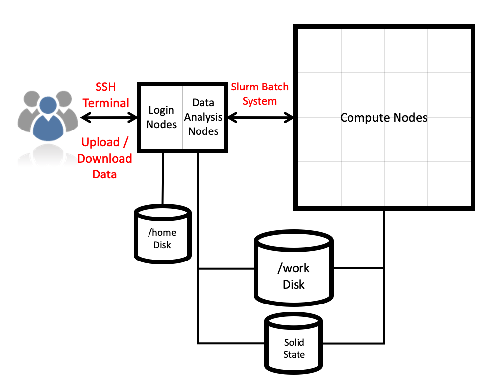
Compute nodes
There are 1,024 compute nodes in total in the 4 cabinet system giving a total of 131,072 compute cores (there will be 5,848 nodes on the full ARCHER2 system, 748,544 compute cores). All compute nodes on the 4 cabinet system with 256 GiB memory per node. All of the compute nodes are linked together using the high-performance Cray Slingshot interconnect.
Access to the compute nodes is controlled by the Slurm scheduling system which supports both batch jobs and interactive jobs.
Storage
There are two different storage systems available on the ARCHER2 4 cabinet system:
- Home
- Work
Home
The home file systems are available on the login nodes only and are designed for the storage of critical source code and data for ARCHER2 users. They are backed-up regularly offsite for disaster recovery purposes. There is a total of 1 PB usable space available on the home file systems.
All users have their own directory on the home file systems at:
/home/<projectID>/<subprojectID>/<userID>
For example, if your username is auser and you are in the project t01 then your home
directory will be at:
/home/t01/t01/auser
Home file system and Home directory
A potential source of confusion is the distinction between the home file system which is the storage system on ARCHER2 used for critical data and your home directory which is a Linux concept of the directory that you are placed into when you first login, that is stored in the
$HOMEenvironment variable and that can be accessed with thecd ~command.
Work
The work file systems, which are available on the login and compute nodes, are designed for high performance parallel access and are the primary location that jobs running on the compute nodes will read data from and write data to. They are based on the Lustre parallel file system technology. The work file systems are not backed up in any way. There will be a total of 14.5 PB usable space available on the work file systems on the final, full ARCHER2 system.
All users have their own directory on the work file systems at:
/work/<projectID>/<subprojectID>/<userID>
For example, if your username is auser and you are in the project t01 then your main home
directory will be at:
/work/t01/t01/auser
Jobs can’t see your data?
If your jobs are having trouble accessing your data make sure you have placed it on Work rather than Home. Remember, the home file systems are not visible from the compute nodes.
More information on ARCHER2 can be found in the ARCHER2 Documentation.
Connecting using SSH
The ARCHER2 login address is
login.archer2.ac.uk
Access to ARCHER2 is via SSH using both a password and a passphrase-protected SSH key pair.
SSH keys
As well as password access, users are required to add the public part of an SSH key pair to access ARCHER2. The public part of the key pair is associated with your account using the SAFE web interface. See the ARCHER2 User and Best Practice Guide for information on how to create SSH key pairs and associate them with your account:
Passwords and password policy
When you first get an ARCHER2 account, you will get a single-use password from the SAFE which you will be asked to change to a password of your choice. Your chosen password must have the required complexity as specified in the ARCHER2 Password Policy.
Logging into ARCHER2
Once you have setup your account in SAFE, uploaded your SSH key to SAFE and retrieved your initial password, you can log into ARCHER2 with:
ssh auser@login.archer2.ac.uk
(Remember to replace auser with your actual username!) On first login, you will be prompted
to change your password from the intial one you got via SAFE, This is a three step process:
- When prompted to enter your LDAP password: Re-enter the password you retrieved from SAFE
- When prompted to enter your new password: type in a new password
- When prompted to re-enter the new password: re-enter the new password
SSH from Windows
While Linux and macOS users can simply use the standard terminal to run the SSH command, this may or may not work from Powershell for Windows users depending on which version of Windows you are using. If you are struggling to connect, we suggest you use MobaXterm.
Log into ARCHER2
If you have not already done so, go ahead and log into ARCHER2. If you run into issues, please let the instructor or helpers know so they can assist.
Key Points
ARCHER2 consists of high performance login nodes, compute nodes, storage systems and interconnect.
The system is based on standard Linux with command line access.
ARCHER2’s login address is
login.archer2.ac.uk.You connect to ARCHER2 using an SSH client.
Break
Overview
Teaching: min
Exercises: minQuestions
Objectives
Comfort break
Key Points
HPC performance and benchmarking
Overview
Teaching: 30 min
Exercises: 25 minQuestions
Why should I benchmark my use of HPC?
What are the key benchmarking concepts that I should understand?
What is the right performance metric for my HPC use?
What parameters can affect the performance of my applications?
Objectives
Understand how benchmarking can improve my use of HPC resources.
Understand key benchmarking concepts and why they are useful for me.
Be able to identify the correct performance metric for my HPC use.
Having looked at workflow components in general we will now move on to look at the specifics of understanding the HPC software component of your workflow to allow you to plan and use your HPC resources more efficiently.
The main tool we are going to use to understand the performance during this course, is benchmarking.
What is benchmarking?
Benchmarking is measuring how the performance of something varies as you change parameters. In our case, we are benchmarking parallel software on HPC systems and so the parameters we will measure performance variation against are usually:
- The number of parallel (usually MPI) processes we use
- The number of threads (usually OpenMP threads) we use
- The distribution of processes/threads across compute nodes
- Any scheduler specific options that affect performance (usually linked to process/thread distribution)
- Calculation input parameters that affect performance
We often want to explore multiple parameters in our benchmarking to get an idea of how performance varies. Needless to say, the search space can become very large!
Why use benchmarking?
Benchmarking your use of software on HPC resources is potentially useful for a range of reasons. These could include:
- Understanding how your current calculations scale to different node/core counts so you can choose the most appropriate setup for your work
- Understanding how your potential future work scales to allow you to request the correct amount of resource in applications for resources
Benchmarking is also commonly used in purchasing new HPC systems to make sure that the new system gives the right level of performance for users. However, you are unlikely to be purchasing your own HPC system so we will not discuss this scenario further here!
Both program and input are important
Remember, it is not just the software package you are benchmarking - it is the combination of the software package and the input data that constitute the benchmark case. Throughout this course we will refer to this combination of the software and the input as the application.
Key benchmarking terminology and concepts
We will use a number of different terms and concepts throughout our discussion on benchmarking so we will define them first:
- Timing: Measured timings for the application you are benchmarking. These timings may be the full runtime of the application or can be timings for part of the runtime, for example, time per iteration or time per SCF cycle.
- Performance: The measure of how well an application is running. Performance is always measured as a rate. The actual unit of performance depends on the application, some common examples are ns/day, iterations/s, simulated years per day, SCF cycles per second. The actual measure you use is the performance metric.
- Baseline performance: Most benchmarking uses a baseline performance to measure performance improvement against. In HPC benchmarking, this will usually be the performance on the smallest number of nodes. (For the extremely simple application we are going to look at, we will actually use a single core but this is often not possible for most real HPC applications.)
- Scaling: A measure of how the performance changes as the number of nodes/cores are increased. Scaling is measured relative to the baseline performance. Perfect scaling is the performance you would expect if there was no parallel overheads in the calculation.
- Parallel efficiency: The ratio of measured scaling to the perfect scaling.
Your application use an benchmarking
Think about your use of HPC. For an HPC application you use, try to identify the timings and performance metric you might use when benchmarking. Why do you think the metrics you have chosen are the correct ones for this case?
Practical considerations
- Plan the benchmark runs you want to perform - what are you planning to measure
and why?
- Remember, you can often vary both input parameters to the application and the parallel distribution on the HPC system itself.
- If you vary multiple parameters at once it can become difficult to interpret the data so you often want to vary one at at time (e.g. number of MPI processes).
- Benchmark performance should be measured multiple times to assess variability.
Three individual runs are usually considered the minimum but more are better.
- We will discuss how to combine multiple runs properly to produce a single value later in the course.
- You should try to capture all of the relevant information on the run as most HPC software do not record these. Details that may not be recorded in the software output may include: environment variables, process/thread distribution, We will talk about how automation can help with this later in the course.
- Organise your output data so that you know which output corresponds to which runs in your benchmark set.
Benchmarking the image sharpening program
Now we will use a simple example HPC application to run some benchmarks and extract timings and performance data. In the next part of this course we will look at how to analyse and present this data to help us interpret the performance of the application.
To do this, we will run the image sharpening program on different numbers of MPI processes for the same input to look at how well its performance scales.
Initial setup
Log into ARCHER2, if you are not already logged in, and load the training/sharpen
module to gain access to the software and input data:
module load training/sharpen
Once this is done, move to your /work directory, create a sub-directory to
contain our benchmarking results and move into it (remember to replace
t001 with the correct project code for your course and auser with your
username on ARCHER2).
Only work file system is visible on the compute nodes
Remember, the work file system is the only one available on the ARCHER2 compute nodes. All just should be launched from a directory on the work file system to ensure they run correctly.
cd /work/t001/t001/auser
mkdir sharpen-bench
cd sharpen-bench
Copy the input data from the central location to your directory:
cp $SHARPEN_INPUT/fuzzy.pgm .
ls
fuzzy.pgm
Baseline performance
For this small example, we are going to use a run on a single core of a compute node as our baseline.
Baseline size
Remember that for real parallel applications, it will often not be possible to use a single core or even a single node as your baseline (due to memory requirements or fitting the run within a reasonable runtime). Nevertheless, you should try and use the smallest size that you feasibly can for your baseline.
Run the single core calculation on an ARCHER2 compute node with:
srun --partition=standard --qos=standard --reservation=ta012_89 --account=ta012 --hint=nomultithread --distribution=block:block --nodes=1 --ntasks-per-node=1 --time=0:10:0 sharpen-mpi.x > sharpen_1core_001.out
srun: job 62318 queued and waiting for resources
srun: job 62318 has been allocated resources
Using srun in this way launches the application on a compute nodes with the
specified resources.
This line is quite long and is going to be tedious to type out each time we want to run a calculation so we will setup a command alias with the options that will not change each time we run to make things easier:
alias srunopt="srun --partition=standard --qos=standard --reservation=ta012_89 --account=ta012 --hint=nomultithread --distribution=block:block"
Making the alias permanent
If you want this alias to persist and be available each time you log into ARCHER2 then you can add the
aliascommand above to the end of your~/.bashrcfile on ARCHER2.
Now we can run the baseline calculation again with:
srunopt --time=0:10:0 --nodes=1 --ntasks-per-node=1 sharpen-mpi.x > sharpen_1core_002.out
srun: job 62321 queued and waiting for resources
srun: job 62321 has been allocated resources
Run the baseline calculation one more time so that we have three separate results.
Lets take a look at the output from one of our baseline runs:
cat sharpen_1core_001.out
 Image sharpening code running on  1 process(es)
 Input file is: fuzzy.pgm
 Image size is: 564 x 770 pixels

 Using a filter of size 17 x  17 pixels
 Reading image file: fuzzy.pgm
 ... done

 Starting calculation ...
Rank 0 on core 0 of node <nid001961>
 .. finished

 Writing output file: sharpened.pgm

 ... done

 Calculation time was  2.882 seconds
 Overall run time was  3.182 seconds
You can see that the output reports various parameters. In terms of timing and performance metrics, the ones of interest to us are:
- Image size: 564 x 770 pixels - this is the size of the image that has been processed.
- Calculation time: 2.882s - this is the time to perform the actual computation.
- Overall run time: 3.182s - this is the total time including the calculation time and the setup/finalisation time (which is dominated by reading the input image and writing the output image).
Based on these parameters, we can propose two timing and corresponding performance metrics:
- Calculation time (in s) and calculation performance (in Mpixels/s): computed as calculation time divided by image size in Mpixels.
- Overall time (in s) and Overall performance (in Mpixels/s): computed as the overall time and divided by the image size in Mpixels.
So, for the output above:
- Image size in Mpixels = (564 * 770) / 1,000,000 = 0.43428 Mpixels
- Calculation time = 2.882s
- Overall time = 3.182s
- Calculation performance = 0.43428 / 2.882 = 0.151 Mpixels/s
- Overall performance = 0.43428 / 3.182 = 0.136 Mpixels/s
Combining multiple runs
Of course, we have three sets of data for our baseline rather than just the single result. What is the best way to combine these to produce our final performance metric?
The answer depends on what you are measuring and why. Some examples:
- You want an idea of the worst case to allow you to be conservative when requesting resources for future applications to make sure you do not run out. In this case, you likely want to use the worst performance at each of your relevant values (core counts for our Sharpening example).
- You want an idea of what the likely amount of work you are going to
get through with the current resources you have. In this case, you will
likely want to take the arithmetic mean of the timings you have and convert this
into the performance metric.
- Note that you should not generally combine rate metric results using the arithmetic mean as this can lead to incorrect conclusions. It is better to combine results using the timings and the convert this result into the rate. (If you need to combine rate metrics, you can use the harmonic mean rather than the arithmetic mean.) See Scientific Benchmarking of Parallel Computing Systems for more information on how to report performance data.)
- You want an idea of the best case scenario to allow you to compare the performance of different HPC systems or parameter choices. In this case, you will likely want to take the best performance at each of your relevant values (core counts for our Sharpening example).
- You want an idea of the performance variation. In this case, you will likely look at the differences between the best and worst performance values, maybe as a percentage of the mean performance.
In this case, we are interested in the change in performance as we change the
number of MPI processes (or cores used) so we will use the minimum timing value
from the multiple runs (as this corresponds to the maximum measured performance).
You can look at this more conveniently using the grep command:
grep time *.out
sharpen_1core_001.out: Calculation time was  2.882 seconds
sharpen_1core_001.out: Overall run time was  3.182 seconds
sharpen_1core_002.out: Calculation time was  2.857 seconds
sharpen_1core_002.out: Overall run time was  3.118 seconds
sharpen_1core_003.out: Calculation time was  2.844 seconds
sharpen_1core_003.out: Overall run time was  3.096 seconds
In my case, the best performance (lowest timing) was from run number 3.
To make the process of extracting the timings and performance data
from the sharpen output files easier for you we have written a small
Python program: sharpen-data.py. This program takes the extension
of the output files (“out” in our examples above), extracts the
data required to compute performance (image size and timings) and
saves them in a CSV (comma-separated values) file.
sharpen-data.py out
Cores        Size      Calc   Overall
    1    0.434280     2.844     3.096
    1    0.434280     2.857     3.118
    1    0.434280     2.882     3.182
Now we have our baseline data. Next, we need to collect data on how the timings and performance vary as the number of MPI processes we use for the calculation increases.
Collecting benchmarking data
Building on your experience so far, the next exercise is to collect the benchmark data we will analyse in the next section of the course.
Benchmarking the performance of Sharpen
Run a set of calculations to benchmark the performance of the
sharpen-mpi.xprogram with the same input up to 2 full nodes (256 cores). Make sure you keep the program output in a suitable set of output files that you can use with thesharpen-data.pyprogram. If you prefer, you can write a job submission script to run these benchmark calculations rather than usingsrundirectly.Solution
People often use doubling of the number of MPI processes as a useful first place for a set of benchmark runs. Going from 1 MPI process to 256 MPI processes this gives the following runs: 2, 4, 8, 16, 32, 64, 128 and 256 MPI processes.
Cores        Size      Calc   Overall
   16    0.434280     0.181     0.450
    2    0.434280     1.432     1.684
    4    0.434280     0.727     0.982
  256    0.434280     0.016     0.310
  128    0.434280     0.029     0.314
   64    0.434280     0.053     0.326
    1    0.434280     2.844     3.096
  256    0.434280     0.016     0.314
   32    0.434280     0.093     0.362
    8    0.434280     0.360     0.615
    8    0.434280     0.360     0.618
  128    0.434280     0.029     0.316
   64    0.434280     0.053     0.327
   32    0.434280     0.093     0.364
    2    0.434280     1.446     1.770
    2    0.434280     1.432     1.685
    4    0.434280     0.727     0.984
   16    0.434280     0.187     0.457
    1    0.434280     2.857     3.118
   32    0.434280     0.094     0.363
  256    0.434280     0.016     0.309
    8    0.434280     0.359     0.617
    4    0.434280     0.717     0.970
   16    0.434280     0.181     0.450
   64    0.434280     0.053     0.322
    1    0.434280     2.882     3.182
  128    0.434280     0.029     0.380
Aggregating data
Next we want to aggregate the data from our multiple runs at particular core counts - remember that, in this case, we want the minimum timing (maximum performance) from the runs to use to compute the performance. To complete these steps we are going to make use of the VisiData tool which allows us to manipulate and visualise tabular data in the terminal.
As well as printing the timing data to the screen, the sharpen-data.py program also
produces a file called benchmark_runs.csv with the data in CSV (comma-separated value)
format that we can use with VisiData. Let’s load the timing data into VisiData:
module load cray-python
module load visidata
vd benchmark_runs.csv
 Cores | Size     | Calc  | Overall ║
 16    | 0.434280 | 0.181 | 0.450   ║
 2     | 0.434280 | 1.432 | 1.684   ║
 4     | 0.434280 | 0.727 | 0.982   ║
 256   | 0.434280 | 0.016 | 0.310   ║
 128   | 0.434280 | 0.029 | 0.314   ║
 64    | 0.434280 | 0.053 | 0.326   ║
 1     | 0.434280 | 2.844 | 3.096   ║
 256   | 0.434280 | 0.016 | 0.314   ║
 32    | 0.434280 | 0.093 | 0.362   ║
 8     | 0.434280 | 0.360 | 0.615   ║
 8     | 0.434280 | 0.360 | 0.618   ║
 128   | 0.434280 | 0.029 | 0.316   ║
 64    | 0.434280 | 0.053 | 0.327   ║
 32    | 0.434280 | 0.093 | 0.364   ║
 2     | 0.434280 | 1.446 | 1.770   ║
 2     | 0.434280 | 1.432 | 1.685   ║
 4     | 0.434280 | 0.727 | 0.984   ║
 16    | 0.434280 | 0.187 | 0.457   ║
 1     | 0.434280 | 2.857 | 3.118   ║
 32    | 0.434280 | 0.094 | 0.363   ║
 256   | 0.434280 | 0.016 | 0.309   ║
1› benchmark_runs| user_macros | saul.pw/VisiData v2.1 | opening benchmark_runs.csv a           27 rows
Your terminal will now show a spreadsheet interface with the timing data from your benchmark runs. You can navigate between different cells using the arrow keys on your keyboard or by using your mouse.
We are now going to use VisiData to aggregate the timing data from our runs. To do this, we first need to let the tool know what type of numerical data is in each of the columns.
Select the “Cores” column and hit # to set it as integer data,
next select the “Size” column and hit % to set it as floating point
data; select the “Calc” column and hit % to set it as
floating point data too; finally, select the “Overall” column and hit % to
set it as floating point data. Your terminal should now look something like:
 Cores#| Size    %| Calc %| Overall%║
    16 |     0.43 |  0.18 |    0.45 ║
     2 |     0.43 |  1.43 |    1.68 ║
     4 |     0.43 |  0.73 |    0.98 ║
   256 |     0.43 |  0.02 |    0.31 ║
   128 |     0.43 |  0.03 |    0.31 ║
    64 |     0.43 |  0.05 |    0.33 ║
     1 |     0.43 |  2.84 |    3.10 ║
   256 |     0.43 |  0.02 |    0.31 ║
    32 |     0.43 |  0.09 |    0.36 ║
     8 |     0.43 |  0.36 |    0.61 ║
     8 |     0.43 |  0.36 |    0.62 ║
   128 |     0.43 |  0.03 |    0.32 ║
    64 |     0.43 |  0.05 |    0.33 ║
    32 |     0.43 |  0.09 |    0.36 ║
     2 |     0.43 |  1.45 |    1.77 ║
     2 |     0.43 |  1.43 |    1.69 ║
     4 |     0.43 |  0.73 |    0.98 ║
    16 |     0.43 |  0.19 |    0.46 ║
     1 |     0.43 |  2.86 |    3.12 ║
    32 |     0.43 |  0.09 |    0.36 ║
   256 |     0.43 |  0.02 |    0.31 ║
1› benchmark_runs|                                                         %  type-float        27 rows
Next, we want to tell VisiData how to aggregate the data in each of the columns. Remember,
we want the minimum value of the timings from the “Calc” and “Overall” columns. Highlight
the “Calc” column and hit +, select min from the list of aggregators and press Return.
Do the same for the “Overall” column. We also want to keep the size value in our aggregated
table so select an aggregator for that column too (min or max are fine here as every row
has the same value). Once you have set the aggregators, select the “Cores” column and
hit “Shift+f” to perform the aggregation. You should see a new table that looks something
like:
 Cores#║ count♯| Size_min%| Calc_min%| Overall_min%║
    16 ║     3 |     0.43 |     0.18 |        0.45 ║
     2 ║     3 |     0.43 |     1.43 |        1.68 ║
     4 ║     3 |     0.43 |     0.72 |        0.97 ║
   256 ║     3 |     0.43 |     0.02 |        0.31 ║
   128 ║     3 |     0.43 |     0.03 |        0.31 ║
    64 ║     3 |     0.43 |     0.05 |        0.32 ║
     1 ║     3 |     0.43 |     2.84 |        3.10 ║
    32 ║     3 |     0.43 |     0.09 |        0.36 ║
     8 ║     3 |     0.43 |     0.36 |        0.61 ║

2› benchmark_runs_Cores_freq|                                                        F           9 bins
The final detail to tidy the aggregated data up before we save it, is to sort by
increasing core count. Select the “Cores” column and hit [ to sort ascending.
Finally, we will save this aggregated data as another CSV file. Hit “Ctrl+s” and
change the file name to benchmark_agg.csv). Now, you can exit VisiData by typing
gq. We will use this CSV file in the next section to compute the performance.
Computing performance
Load up VisiData again with the aggregate timing data:
vd benchmark_agg.csv
 Cores | count | Size_min | Calc_min | Overall_min ║
 1     | 3     | 0.43     | 2.84     | 3.10        ║
 2     | 3     | 0.43     | 1.43     | 1.68        ║
 4     | 3     | 0.43     | 0.72     | 0.97        ║
 8     | 3     | 0.43     | 0.36     | 0.61        ║
 16    | 3     | 0.43     | 0.18     | 0.45        ║
 32    | 3     | 0.43     | 0.09     | 0.36        ║
 64    | 3     | 0.43     | 0.05     | 0.32        ║
 128   | 3     | 0.43     | 0.03     | 0.31        ║
 256   | 3     | 0.43     | 0.02     | 0.31        ║

1› benchmark_agg| user_macros | saul.pw/VisiData v2.1 | opening benchmark_agg.csv as             9 rows
Now we are going to create new columns with the performance (in Mpixels/s) which we will use in the next section when we analyse the data.
The maximum calculation performance is computed as the size divided by the minimum
calculation timing. We can use VisiData to compute this for us but first we need to
tell the tool what numerical data is in each column (as we did for aggregating the
data, if we had not quit VisiData, we could skip this step). So, set the Cores
column as integer data (using #) and the other columns as floating point data
(using %).
Now, select the “Calc_min” column and hit =, VisiData now asks us for a formula
to use to compute a new column. Enter Size_min / Calc_min. This should create
a new column with the performance:
 Cores#| count | Size_min%| Calc_min%| Size_min/Calc_min  | Overall_min%║
     1 | 3     |     0.43 |     2.84 | 0.151408450704225…%|        3.10 ║
     2 | 3     |     0.43 |     1.43 | 0.300699300699300…%|        1.68 ║
     4 | 3     |     0.43 |     0.72 | 0.5972222222222222%|        0.97 ║
     8 | 3     |     0.43 |     0.36 | 1.1944444444444444%|        0.61 ║
    16 | 3     |     0.43 |     0.18 | 2.388888888888889 %|        0.45 ║
    32 | 3     |     0.43 |     0.09 | 4.777777777777778 %|        0.36 ║
    64 | 3     |     0.43 |     0.05 | 8.6               %|        0.32 ║
   128 | 3     |     0.43 |     0.03 | 14.333333333333334%|        0.31 ║
   256 | 3     |     0.43 |     0.02 | 21.5              %|        0.31 ║

1› benchmark_agg|                                        BUTTON1_RELEASED  release-mouse         9 rows
Move to the new column and set it to floating point data. We can also rename
the column to be more descriptive: hit ^ and give it the name Calc_perf_max.
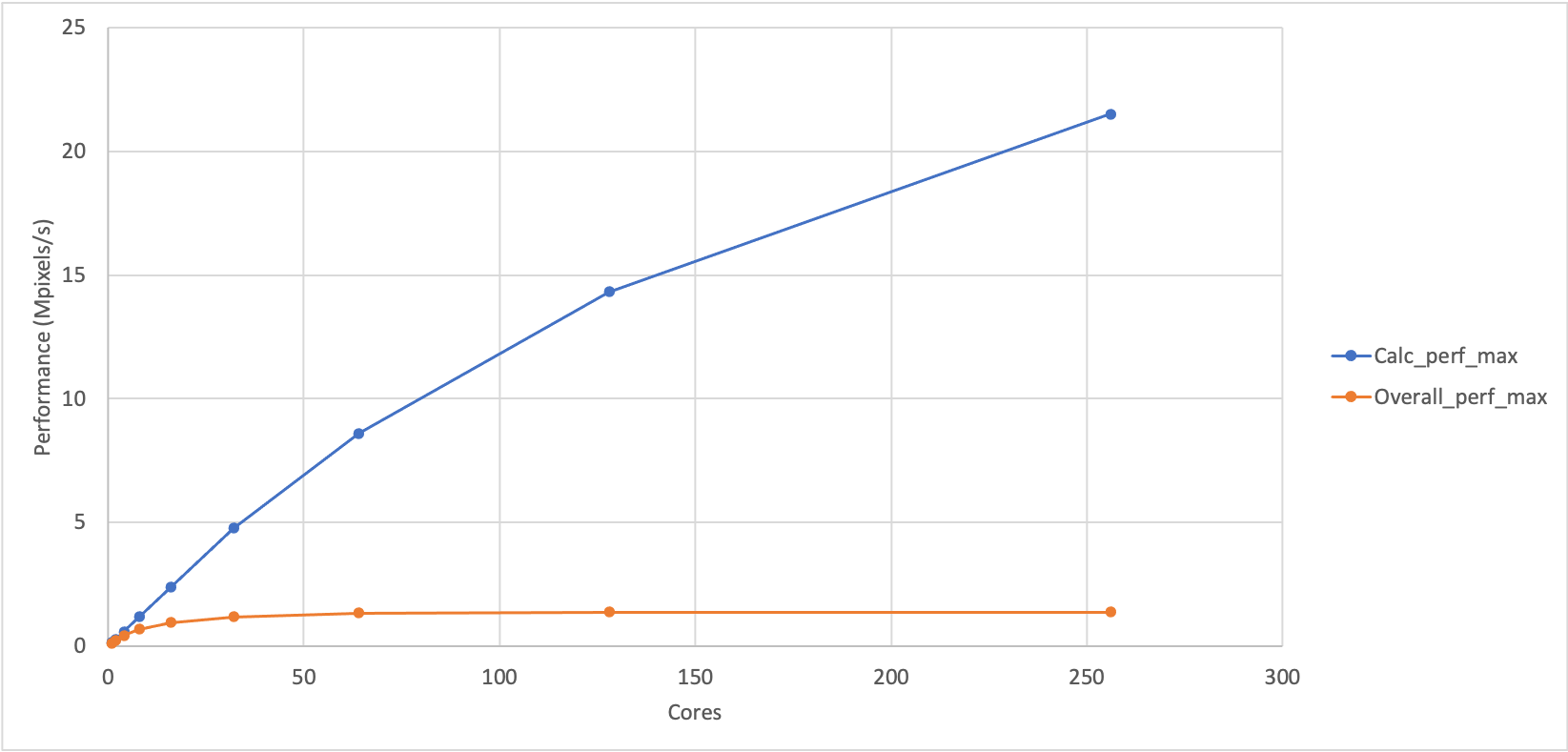
 Cores#| count | Size_min%| Calc_min%| Calc_perf_max     %| Overall_min%║
     1 | 3     |     0.43 |     2.84 |               0.15 |        3.10 ║
     2 | 3     |     0.43 |     1.43 |               0.30 |        1.68 ║
     4 | 3     |     0.43 |     0.72 |               0.60 |        0.97 ║
     8 | 3     |     0.43 |     0.36 |               1.19 |        0.61 ║
    16 | 3     |     0.43 |     0.18 |               2.39 |        0.45 ║
    32 | 3     |     0.43 |     0.09 |               4.78 |        0.36 ║
    64 | 3     |     0.43 |     0.05 |               8.60 |        0.32 ║
   128 | 3     |     0.43 |     0.03 |              14.33 |        0.31 ║
   256 | 3     |     0.43 |     0.02 |              21.50 |        0.31 ║

1› benchmark_agg|                                        BUTTON1_RELEASED  release-mouse         9 rows
Compute the Overall maximum performance at each core count
Add a column called
Overall_perf_maxthat contains the Overall maximum performance at each core count and that is formatted as floating point values.Solution
Select the “Overall_min” column and hit
=, VisiData now asks us for a formula to use to compute a new column. EnterSize_min / Overall_min. Move to the new column and hit%to format it as floating point values and then hit^to rename itOverall_perf_max. The final table should look something like:Cores#| count | Size_min%| Calc_min%| Calc_perf_max %| Overall_min%| Overall_perf_max %║ 1 | 3 | 0.43 | 2.84 | 0.15 | 3.10 | 0.14 ║ 2 | 3 | 0.43 | 1.43 | 0.30 | 1.68 | 0.26 ║ 4 | 3 | 0.43 | 0.72 | 0.60 | 0.97 | 0.44 ║ 8 | 3 | 0.43 | 0.36 | 1.19 | 0.61 | 0.70 ║ 16 | 3 | 0.43 | 0.18 | 2.39 | 0.45 | 0.96 ║ 32 | 3 | 0.43 | 0.09 | 4.78 | 0.36 | 1.19 ║ 64 | 3 | 0.43 | 0.05 | 8.60 | 0.32 | 1.34 ║ 128 | 3 | 0.43 | 0.03 | 14.33 | 0.31 | 1.39 ║ 256 | 3 | 0.43 | 0.02 | 21.50 | 0.31 | 1.39 ║ 1› benchmark_agg| "Overall_perf_max" ^ rename-col 9 rows
Finally, save this data in a CSV file called benchmark_perf.csv and exit VisiData.
Why do you want to use benchmarking
Think about your use of HPC. What would you want to get out of benchmarking? Would measuring the minimum, maximum, mean or performance variation be appropriate for what you want to do and why?
What parameters would you be interested in varying for the application you want to benchmark?
Capturing run details
As for determining what the correct performance measure is (min, max, mean), the choice of what details of the benchmark run to capture depend on what you are measuring performance against and why. If the output does not include the values you require automatically then you should ensure it is captured in some way.
Here are some concrete examples of scenarios and the information you should ensure is captured:
- Comparing performance as a function of number of cores/nodes on a particular HPC system - In this case you need to ensure that the output captures the number of cores, nodes, MPI processes, OpenMP threads (depending on what varies). Most applications will include this information somewhere in their output.
- Comparing performance as input parameters change - In this case you must ensure that the output captures the value of the input parameters that are changing. These are usually captured in the output by the application itself.
- Comparing performance of applications compiled in different ways - You may be comparing the performance of different versions of an application or those compiled using different compilers or with different compile-time options. These differences will not usually be captured by the application itself and so should be captured by yourself in the output in some way (this could be by the name of the directory or files the output is in or by adding details to the output as part of the benchmark run.)
- Comparing performance across different HPC systems- This is the most difficult as there is often a lot of differences to capture across different HPC systems. You usually need to capture all of the details that have been mentioned for the previous cases along with other details such as the run time environment and the hardware details of the different systems.
As with all the aspects we have discussed so far, you should plan in advance the details that need to be captured as part of your benchmarking activity and how they will be captured so you do not need to re-run calculations because you do not have a good record of the differences between runs.
Summary
In this section we have discussed:
- Basic benchmarking terminology
- The difference between timings and performance measures (rates)
- Selecting performance metrics
- Running benchmark calculations and gathering data
- Capturing information on differences between benchmark runs
We also used a simple example application to allow us to collect some benchmark data on ARCHER2.
Now we have collected our benchmarking data we will turn to how to analyse the data, understand the performance and make decisions based on it.
Key Points
Different timing and performance metrics are used for different applications.
Use the lowest node/core count that is feasible for your baseline.
Plan your benchmarking before you start, make sure you understand which parameters you want to vary and why.
Analysing performance
Overview
Teaching: 30 min
Exercises: 30 minQuestions
How do I analyse the results of my benchmarking?
Which metrics can I use to make decisions about the best way to run my calculations?
What are the aspects I should consider when making decisions about parallel performance?
What stops my HPC use from scaling to higher node counts?
Objectives
Understand how to analyse and understand the performance of your HPC use.
Understand speedup and parallel efficiency metrics and how they can support decisions.
Have an awareness of the limits of parallel scaling: Amdahl’s Law and Gustafson’s Law.
In the last section we talked about performance metrics and how to gather benchmark data and used an simple example program as an example. In this section we will look at how to analyse the data we have gathered, start to understand performance and how to use the analysis to make decisions.
Plotting performance
As well as providing a spreadsheet interface to allow us to manipulate data, VisiData also allows us to produce scatter plots in the terminal to quickly look at how the performance varies with core count.
First, let’s load the performance data into VisiData again:
module load cray-python
module load visidata
vd benchmark_perf.csv
 Cores | count | Size_min | Calc_min | Calc_perf_max | Overall_min | Overall_perf_max ║
 1     | 3     | 0.43     | 2.84     | 0.15          | 3.10        | 0.14             ║
 2     | 3     | 0.43     | 1.43     | 0.30          | 1.68        | 0.26             ║
 4     | 3     | 0.43     | 0.72     | 0.60          | 0.97        | 0.44             ║
 8     | 3     | 0.43     | 0.36     | 1.19          | 0.61        | 0.70             ║
 16    | 3     | 0.43     | 0.18     | 2.39          | 0.45        | 0.96             ║
 32    | 3     | 0.43     | 0.09     | 4.78          | 0.36        | 1.19             ║
 64    | 3     | 0.43     | 0.05     | 8.60          | 0.32        | 1.34             ║
 128   | 3     | 0.43     | 0.03     | 14.33         | 0.31        | 1.39             ║
 256   | 3     | 0.43     | 0.02     | 21.50         | 0.31        | 1.39             ║

1› benchmark_perf|                                     KEY_RESIZE  redraw         9 rows
As noted earlier, VisiData allows us to show scatter plots in the terminal to get a quick visual representation of the relationship between the data in different columns. To do this, we need to make sure the columns are set to the correct numerical data types and say which one is going to be the x-axis.
Select the “Cores” column and hit # to set it as integer data,
next select the “Calc_perf_max” column and hit % to set it as floating point
data, finally select the “Overall_perf_max” column and hit % to set it as
floating point data too. Your terminal should now look something like:
 Cores#| count | Size_min | Calc_min | Calc_perf_max%| Overall_min | Overall_perf_max%║
     1 | 3     | 0.43     | 2.84     |          0.15 | 3.10        |             0.14 ║
     2 | 3     | 0.43     | 1.43     |          0.30 | 1.68        |             0.26 ║
     4 | 3     | 0.43     | 0.72     |          0.60 | 0.97        |             0.44 ║
     8 | 3     | 0.43     | 0.36     |          1.19 | 0.61        |             0.70 ║
    16 | 3     | 0.43     | 0.18     |          2.39 | 0.45        |             0.96 ║
    32 | 3     | 0.43     | 0.09     |          4.78 | 0.36        |             1.19 ║
    64 | 3     | 0.43     | 0.05     |          8.60 | 0.32        |             1.34 ║
   128 | 3     | 0.43     | 0.03     |         14.33 | 0.31        |             1.39 ║
   256 | 3     | 0.43     | 0.02     |         21.50 | 0.31        |             1.39 ║

1› benchmark_perf|                                          %  type-float         9 rows
Now we will set the “Cores” column as the x-axis variable. Select the “Cores”
column and hit ! - it should change colour (it is now blue in my terminal)
to show it has been set as the categorical data.
Finally, we can plot the graph by hitting g. (g followed by a period). You
should see something like the plot shown below which shows the variation of
maximum performance for the calculation part of Sharpen and the overall
performance of Sharpen (calculation and IO). (We have also included a plot
of the same data in Excel as it is difficult to see the terminal plot in the
web interface for the course.)
21.50                                                                 1:Calc_perf_max ⠁
                                                                      2:Overall_perf_max


16.16

                                                ⠂


10.82


                             ⠂


5.48
                   ⠁

              ⠠
            ⡀      ⡀         ⠄                  ⠄                                     ⠄
0.14      ⢠⠆⠂ ⠈
Cores»    1                  64                 128                192                256
2› benchmark_perf_graph| loading data points | loaded 18 points (0  g.          18 plots
Plotting timing data
Use Visidata to plot the timing data rather than the peformance. Looking at the timing plot, can you think of a reason why plotting the performance data is often preferred over plotting the raw timing data.
What does this show?
You can see that the performance of the calculation part and the overall performance look different. Can you come up with any explanation for the difference in performance?
Solution
If the overall calculation was just dependent on the performance of the sharpening calculation then it would show similar performance trends to calculation part. This indicates that there is something else in the sharpen program that is adversely affecting the performance as we increase the number of cores.
Analysis
We are going to analyse our benchmark data for the Sharpen example by looking at two metrics that we introduced earlier:
- Speedup: The ratio of performance at a particular core count relative to our baseline performance.
- Parallel efficiency: The percentage of perfect speedup that we observe at a
- particular core count.
Speedup
Compute the speedup for the maximum calculation and maximum overall performance
Using the data you have, compute the speedup for the maximum calculation and maximum overall performance. You can do this by hand, by using VisiData (this is what the solution will demonstrate), by downloading the CSV and using a spreadsheet software on your laptop (e.g. Excel) or by writing a script. Remember that the speedup is the ratio of performance to the baseline performance.
You should also add a column with the values for perfect speedup. As our baseline performance is measured on a single core, the perfect speedup is actually just the same as the number of cores in this case.
Finally, can you produce a plot showing the calculation speedup, the overall speedup and the perfect speedup?
In VisiData, you can create a column of data based on data in other columns by moving to the column to the left of where you want the new column to be, typing
=to start an expression and using the column names in the expression. For example, to produce a column that had all the data in the “Calc_perf_max” column divided by the value in the first row from “Calc_perf_max” (which, in my case, is 0.15) then you would enter=Calc_perf_max/0.15. You can rename a column by hitting^when the column you want to rename is selected. Remember, you will need to set the column data type before you can plot it. You can exclude columns from plots by hiding them by highlighting the column and hitting-. You can unhide all columns once you have finished plotting withgv.Solution
Computing speedup
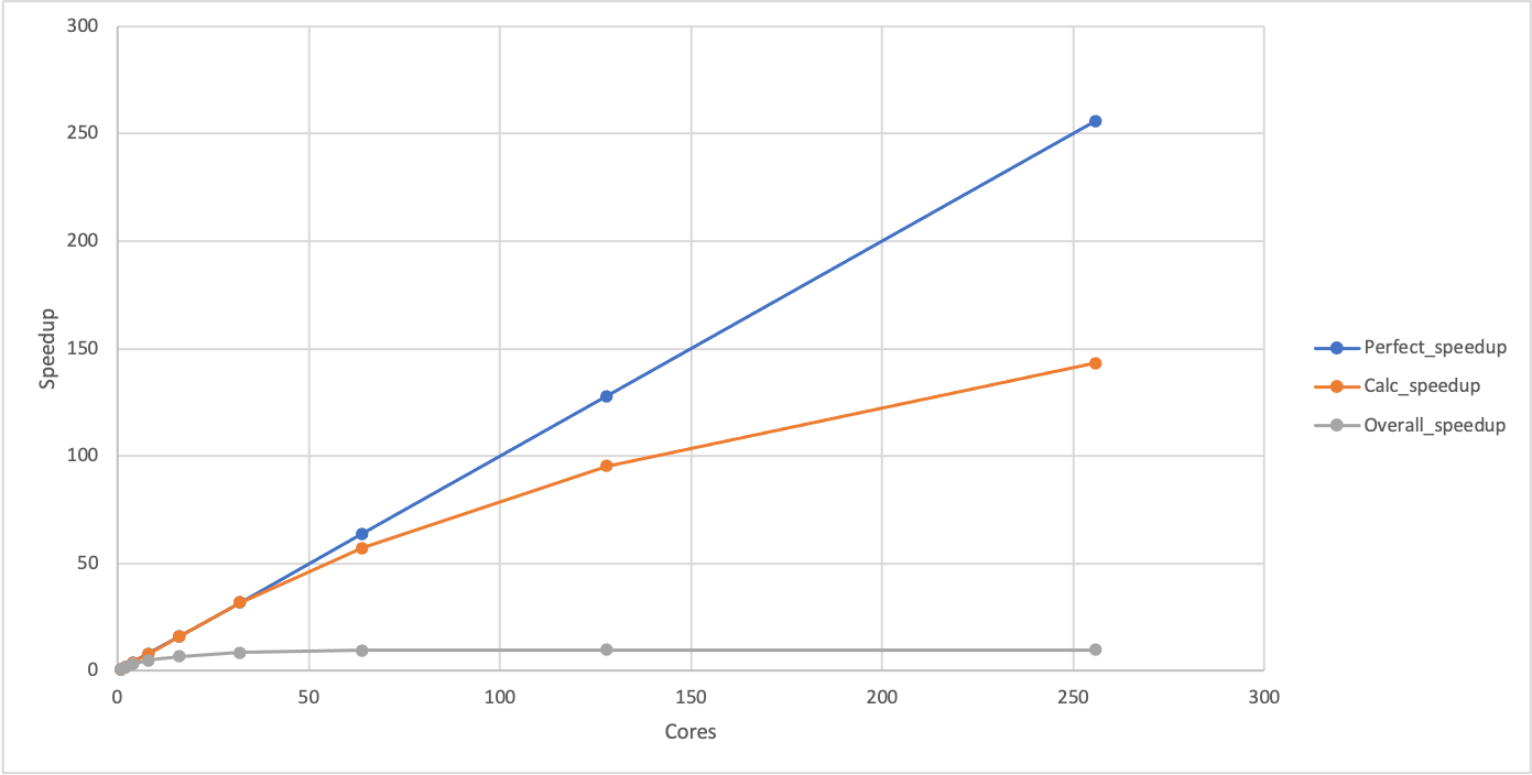
Note the value for the “Calc_perf_max” on one core - this is the baseline performance we are going to use to compute the speedup, in my case it is 0.15. Highlight the “Calc_perf_max” column and create a new column with the speedup by entering
=Calc_perf_max/0.15and press enter (remember to replace 0.15 with your baseline performance). This should create a new column with the speedup. Highlight that column and hit%to set it as floating point data. Use^to rename the column asCalc_speedup. Repeat the process for the “Overall_perf_max” column (remember to use its baseline rather than the Calc baseline). Add a perfect speedup column by highlighting the “Cores” column and then entering=Coresand pressing enter. Change the name of this column to “Perfect_speedup” and set to integer data. Once you have done this, you should have a spreadsheet that looks something like (note some columns have scrolled off the right of my terminal):Cores#| Perfe#| count | Size_min | Calc_min | Calc_perf_max%| Calc_speedup %| Over> 1 | 1 | 3 | 0.43 | 2.84 | 0.15 | 1.00 | 3.10 2 | 2 | 3 | 0.43 | 1.43 | 0.30 | 2.00 | 1.68 4 | 4 | 3 | 0.43 | 0.72 | 0.60 | 4.00 | 0.97 8 | 8 | 3 | 0.43 | 0.36 | 1.19 | 7.93 | 0.61 16 | 16 | 3 | 0.43 | 0.18 | 2.39 | 15.93 | 0.45 32 | 32 | 3 | 0.43 | 0.09 | 4.78 | 31.87 | 0.36 64 | 64 | 3 | 0.43 | 0.05 | 8.60 | 57.33 | 0.32 128 | 128 | 3 | 0.43 | 0.03 | 14.33 | 95.53 | 0.31 256 | 256 | 3 | 0.43 | 0.02 | 21.50 | 143.33 | 0.31 1› benchmark_perf| KEY_LEFT go-left 9 rowsAt this point, you should save the file as
benchmark_speedup.csv.Plot speedup
Hide the “Calc_perf_max” and “Overall_perf_max” columns by highlighting them one at a time and hitting
-. Highlight the “Cores” column and hit!to set it as the categorical data. This should show a plot that looks something like:256 1:Perfect_speedup 2:Calc_speedup 3:Overall_speedup 192 ⠄ 128 ⠁ ⡀ 64 ⠄ ⠁ ⠁ ⠠ 1 ⢀⠄⠆ ⠐ ⠁ ⠁ ⠁ ⠁ Cores» 1 64 128 192 256 3› benchmark_perf_graph| loading data points | loaded 27 points (0 g. 27 plotsYou can see that the calculation speedup is much closer to the perfect scaling than the overall speedup. You can use
qto get back to the spreadsheet view andgvto unhide the hidden columns.
Speedup and performance
If plotted, the speedup should show the same shape as the performance plot we produced earlier with the difference that it will start at 1 for a single core (where the baseline and the observed performance are identical). Given this, Why do we use the two different metrics in our analysis? In short, we do not have to, but it can be more convenient to work with speedup rather than performance when comparing to ideal parallel performance and it is also a useful step towards computing the parallel efficiency which is often a key dimensionless decision-making metric.
Plotting performance directly is generally better for showing the differences between different setups (e.g. different HPC systems, different software versions) as it avoids the choice of baseline that must be made when plotting speedup and gives a better indication of the absolute performance differences between the different setups.
Parallel efficiency
Now we have columns with the calculated speedups and perfect speedup we can use these to compute the parallel efficiency which is often a better metric for making decisions about what the right scale to run calculations.
Calculate the parallel efficiency
Add columns to your spreadsheet (or output if you wrote a script) that show the calculation parallel efficiency and the overall parallel efficiency. Remember, the parallel efficiency is the ratio of the observed speedup to the perfect speedup.
Given the parallel efficiencies you have calculated can you propose a maximum core count that can be usefully used for this Sharpen example - both in terms of overall and in terms of just the calculation part? Why did you choose these values?
Solution
We will illustrate the solution using VisiData. Select the “Calc_speedup” column and setup a new computed column using
=Calc_speedup/Perfect_speedup, Select the new column and set it as floating point and change the column name to “Calc_efficiency”. Do the same for the “Overall_speedup”. Once you have done this, you should have something that looks like (note some columns have scrolled off the right of my terminal):Cores#║ Perfe#| count | Size_min | Calc_min | Calc_speedup %| Calc_effciency %|> 1 ║ 1 | 3 | 0.43 | 2.84 | 1.00 | 1.00 |… 2 ║ 2 | 3 | 0.43 | 1.43 | 2.00 | 1.00 |… 4 ║ 4 | 3 | 0.43 | 0.72 | 4.00 | 1.00 |… 8 ║ 8 | 3 | 0.43 | 0.36 | 7.93 | 0.99 |… 16 ║ 16 | 3 | 0.43 | 0.18 | 15.93 | 1.00 |… 32 ║ 32 | 3 | 0.43 | 0.09 | 31.87 | 1.00 |… 64 ║ 64 | 3 | 0.43 | 0.05 | 57.33 | 0.90 |… 128 ║ 128 | 3 | 0.43 | 0.03 | 95.53 | 0.75 |… 256 ║ 256 | 3 | 0.43 | 0.02 | 143.33 | 0.56 |… 1› benchmark_perf| KEY_LEFT go-left 9 rows8 cores for the overall speedup (63% parallel efficiency) is the limit of useful scaling and 128 cores for the calculation speedup (75% parallel efficiency) is the limit of useful scaling from the values measured.
Anything less than 70% parallel efficiency is generally considered poor scaling and less than 60% parallel efficiency is generally considered not a reasonable use of compute time in normal workflow production. Of course, if the time to solution is critical (for example, responding to an urgent request for data) then it may be acceptable to run with very poor parallel efficiency to achieve a faster time to solution but it should be carefully considered if the compute cycles could be better used by running multiple calculations in parallel rather than the inefficient use of resources by scaling the single calculation beyond its limits. In this case, the overall speedup is not improving at all beyond 64 cores so using more than this is futile anyway.
Limits to scaling/speedup and parallel efficiency
As we have seen with this example, there are often limits to how well a parallel program can scale. By scaling, we mean the ability to use more resources on an HPC system. Most often this refers to nodes or cores but it can also refer to other hardware such as GPU accelerators or IO. In the sharpen case, we are talking about the scaling to higher core counts.
Strong and weak scaling
In HPC, scaling is usually referred to in terms of strong scaling or weak scaling and when interpreting performance data it is important that you know which case you are dealing with.
- Strong Scaling – total problem size stays the same as the amount of of resource (cores in this case) increases.
- Weak Scaling - the problem size increases at the same rate as the amount of HPC resource (cores in this case), keeping the amount of work per resource unit the same.
The image sharpening case we have been using is an example of a strong scaling problem.
Strong scaling is more useful in general and often more difficult to achieve in practice.
Weak scaling image sharpening?
Can you think of how you might use the image sharpening example to look at the weak scaling peformance of the code? What would you have to change about the way we run the program to do this?
The limits of scaling (as we have seen, usually measured in parallel efficiency) in the cases of both strong and weak scaling are well understood. They are captured in Amdahl’s Law (strong scaling) and Gustafson’s Law (weak scaling).
Strong scaling limits: Amdahl’s Law
“The performance improvement to be gained by parallelisation is limited by the proportion of the code which is serial” - Gene Amdahl, 1967
What does this actually mean? We can see what this means from the sharpen example that we have been looking at. The reason that this example stops scaling Overall even though the Calculation part scales well is because there is a serial part of the code (the IO: reading the input and writing the output). Here I have computed the IO time by subtracting the Calculation time from the Overall time. The “IO_min” column shows the time taken for the IO part and the “Fraction_IO” column shows what fraction of the total runtime is taken up by IO.
 Cores | Calc_min%| Overall_min%| IO_min              %| Fraction_IO        %║
 1     |     2.84 |        3.10 |                 0.26 |                0.08 ║
 2     |     1.43 |        1.68 |                 0.25 |                0.15 ║
 4     |     0.72 |        0.97 |                 0.25 |                0.26 ║
 8     |     0.36 |        0.61 |                 0.25 |                0.41 ║
 16    |     0.18 |        0.45 |                 0.27 |                0.60 ║
 32    |     0.09 |        0.36 |                 0.27 |                0.75 ║
 64    |     0.05 |        0.32 |                 0.27 |                0.84 ║
 128   |     0.03 |        0.31 |                 0.28 |                0.90 ║
 256   |     0.02 |        0.31 |                 0.29 |                0.94 ║

1› benchmark_perf|                                  -  hide-col         9 rows
What do we see? The IO time is constant as the number of cores increases, indicating that this part of the code is serial (it does not benefit from more cores). As the number of cores increases, the serial part becomes a larger and larger fraction of the overall run time (the calculation time decreases as it benefits from parallelisation). In the end, it is this serial part of the code that limits the parallel scalability.
Even in the absence of any overheads to parallelisation, the speedup of a parallel code is limited by the fraction of serial work for the application (parallel program + specific input). Specifically, the maximum speedup that can be achieved for any number of parallel resources (cores in our case) is given by 1/α, where α is the fraction of serial work in our application.
If we go back and look at our baseline result at 1 core, we can see that the fraction of serial work (the IO part) is 0.08 so the maximum speedup we can potentially achieve for this application is 1/0.08 = 12.5. The maximum speedup we actually observe in is around 10 (because the parallel section does not parallelise perfectly at larger core counts due to parallel overheads).
Lots of parallelisation needed…
If we could reduce the serial fraction to 0.01 (1%) of the application then we would still be limited to a maximum speedup of 100 no matter how many cores you use. On ARCHER2, there are 128 cores on a node and typical calculations may use more than 1000 cores so you can start to imagine how much work has to go into parallelising applications!
Weak scaling limits: Gustafson’s Law
For weak scaling applications - where the size of the application increases as you increase the amount of HPC resource - the serial component does not dominate in the same way. Gustafson’s Law states that for a number of cores, P, and an application with serial fraction α, the scaling (assuming no parallel overheads) is given by P - α(P-1). For example, for an application with α=0.01 (1% serial) on 1024 cores (8 ARCHER2 nodes) the maximum speedup will be 1013.77 and this will keep increasing as we increase the core count.
If you contrast this to the limits for strong scaling given by Amdahl’s Law for a similar serial fraction of code and you can see why good strong scaling is usually harder to achieve.
Why not always use weak scaling approaches?
Given the better prospects for scaling applications using a weak scaling approach, why do you think this approach is not always used for parallelising applications on HPC systems?
Solution
In many cases, using weak scaling approaches may not be an option for us. Some potential reasons are:
- An increased problem size has no relevance to the work we are doing
- Our time would be better used running multiple copies of smaller systems rather than fewer large calculations
- There is no scope for increasing the problem size
Summary
Now we should have a good handle on how we go about benchmarking performance of applications on HPC systems and how to analyse and understand the performance. In the next section we look at how to automate the collection and analysis of performance data.
Key Points
You can use benchmarking data to make decisions on how to best use your HPC resources.
Parallel efficiency is often the key decision metric for limits of parallel scaling.
Parallel performance is ultimately limited by the serial parts of the calculation.
Lunch
Overview
Teaching: min
Exercises: minQuestions
Objectives
Lunch
Key Points
Automating performance data collection and analysis
Overview
Teaching: 30 min
Exercises: 40 minQuestions
Why is automation useful?
What considerations should I have when automating collecting performance data?
Are there any tools that can help with automation?
Objectives
Understand how automation can help with performance measurements.
See how different automation approaches work in practice.
We now know how to collect basic benchmark performance data and how to analyse it so that we can understand the performance and make decisions based on it. We will now look at techniques for making data collection and analysis more efficient.
Why automate?
The manual collection of benchmark data can become a onerous, time-consuming task, particularly if you have a large parameter space to explore. When you have more than a small number of benchmark runs to undertake it is often worthwhile automating the collection of benchmarking data.
In addition to reducing the manual work, automation of data collection has a number of other advantages:
- It can make the collection of data more systematic across different parameters
- It can make the recording of details more consistent
- It can simplify the automation of analysis
- It can make it easier to rerun benchmarking in the future (on the same or different systems)
Automation approaches
There are a number of different potential approaches to automation: ranging from using a existing framework to creating your own scripts. The approach you choose generally depends on how many benchmark runs you need to perform and how much data you plan to collect. The larger the dataset you are interested in, the more time it will be worth investing in automation.
Many ways to skin a cat!
Like many programmatic problems, there are an extremely large number of ways to address this problem. We will cover one approach here using bash scripting, but that does not mean you could not use Perl, Python or any other language and approach. Often the best choice depends on what toolset you are already familiar with and happy using.
Automating Sharpen benchmarking
In this lesson, we will look at writing our own simple scripts to automate the collection of benchmark data for the Sharpen application to repeat the work we have already done by hand to demonstrate one potential approach.
First, we need to decide what parameters are varying and if there are any data we need to capture from the runs that will not be captured in the output from the application itself.
Things we need to vary:
- Number of cores
- Run number at this data point
Things we need to capture that are not in the application output:
- Date and time of the run
- Run number at this data point
We have already seen how to use srun directly to run these benchmarks, but in
this case we will generate job submission scripts to run the benchmarks. This is
not strictly needed here, but will demonstrate an approach that is more
flexible for your potential use cases than submitting using srun directly.
Write the template job submission script
Firstly, we want to write a job submission script that will submit one instance of a benchmark run.
Writing a job submission script
Use the ARCHER2 online documentation to produce a job submission script that runs the Sharpen application on a single core on a single node.
Solution
The following job submission script sets the same options that we used when using
srundirectly.#!/bin/bash # Slurm job options (job-name, compute nodes, job time) #SBATCH --job-name=sharpen_bench #SBATCH --time=0:20:0 #SBATCH --nodes=1 #SBATCH --tasks-per-node=1 #SBATCH --cpus-per-task=1 #SBATCH --account=ta012 #SBATCH --partition=standard #SBATCH --qos=standard #SBATCH --reservation=ta012_89 # Setup the job environment (this module needs to be loaded before any other modules) module load epcc-job-env # Load the sharpen module module load training/sharpen srun --distribution=block:block --hint=nomultithread sharpen-mpi.x > bench_${SLURM_NTASKS}cores_run1.out
Identify parameters that will vary in the script and write parameterised submission script
Now, we need to take our static script and identify all the locations where things will change dynamically during automated setup and any additional parameters/data that we need to include. Remember, we thought the following things would change:
- Number of cores
- Run number at this data point
and we need to remember to include these additional data for each run (because they are not included in the output from Sharpen):
- Date and time of the run
- Run number at this data point
Looking at our basic script, we can see that the number of cores appears in the following line:
#SBATCH --tasks-per-node=1
(It may also sometimes require an increase in the number of nodes if we use more cores than are in a single node but we shall ignore this for now.)
The run number does not appear anywhere in our script at the moment, so we will need to find a way to include it. When we do this, it will also address including the run number in the output in some way.
Finally, we need to capture the date/time in a way that can be used in our output. One
convenient way to do this is to capture the time as epoch time (seconds since
1970-01-01 00:00:00 UTC). We can use the command date +%s to get this. So, we could
capture this in a script with something like:
timestamp=$(date +%s)
(This captures the current epoch time into the $timestamp variable. Note that there
cannot be any spaces on either side of the = sign in bash scripts.)
We are going to use a bit of bash scripting to create a version of our job submission script that will allow us to specify the values of the variables that we want to change as arguments and that will include the date. First we will show the complete script and then we will explain what is going on.
Here is the script (which I saved in run_benchmark.sh):
# Capture the arguments
ncores=$1
nruns=$2

sbatch <<EOF
#!/bin/bash

# Slurm job options (job-name, compute nodes, job time)
#SBATCH --job-name=sharpen_bench
#SBATCH --time=0:20:0
#SBATCH --nodes=1
#SBATCH --tasks-per-node=${ncores}
#SBATCH --cpus-per-task=1
#SBATCH --account=ta012
#SBATCH --partition=standard
#SBATCH --qos=standard
#SBATCH --reservation=ta012_89

# Setup the job environment (this module needs to be loaded before any other modules)
module load epcc-job-env
# Load the sharpen module
module load training/sharpen

for irun in \$(seq 1 ${nruns})
do
   timestamp=\$(date +%s)
   srun --distribution=block:block --hint=nomultithread sharpen-mpi.x > bench_\${SLURM_NTASKS}cores_run\${irun}_\${timestamp}.out
done
EOF
To use this script to run three copies of the benchmark on a single core, we would use the command:
bash run_benchmark.sh 1 3
Submitted batch job 65158
The first argument to the script specifies the number of cores and the second argument,
the number of copies to run. In the script itself, these are captured into the
variables $ncores and $nruns by the lines:
ncores=$1
nruns=$2
We then use a form of bash redirection called a here document to pass the script to the sbatch command with the
values of $ncores and $nruns substituted in in the correct places: the SBATCH option
for $ncores and the seq command for $nruns. One thing to note in the here document
is that we must escape the $ for variables we want to still be variables in the
script by preceding them with a backslash otherwise bash will try to substitute them
in the same way it does for the $ncores and $nruns variables. You can see this
in action in the for line, timestamp line and the srun line: we want these variables to be
interpreted when the script runs so they need to be escaped, the unescaped variables
will be interpreted when the script is submitted.
Remember, that the value of the walltime specified for the job now needs to be long enough for however many repeats of the runs we want to run (20 minutes is plenty for the Sharpen application). (You could, of course, calculate this in the script based on a base runtime and the specified number of repeats if you so wish.)
Now we have a script that can dynamically take the values we want for benchmarking, and we already have a script that can automatically extract the data from all benchmark runs, the final step is to setup the script that can automate the submission of the different benchmark cases.
Write the benchmark automation script and submit the jobs
To automate the submission, we need a script that could call our parameterised submission script with the different parameters needed. For this simple case, we will encode the different parameters in the script itself but for more complex cases it may be worth considering keeping the parameters in a separate file that can be read by the script.
In this case, the only parameter we want to vary is the number of cores for the benchmark (we are going to use 3 repetitions per core count). Here is an example of a short bash script that would implement this:
# Set the core counts we want to benchmark
core_counts="1 2 4 8 16 32 64 128"
# Set the number of repeat runs per core count
nrep=3

# Loop over core counts, submitting the jobs
for cores in $core_counts
do
   bash run_benchmark.sh $cores $nrep
done
Assuming this has been saved as launch_benchmark.sh in the same directory as our
run_benchmark.sh script, we should now be able to submit the full set of benchmark
runs with a single command:
bash launch_benchmark.sh
Submitted batch job 65174
Submitted batch job 65175
Submitted batch job 65176
Submitted batch job 65177
Submitted batch job 65178
Submitted batch job 65179
Submitted batch job 65180
Submitted batch job 65181
You can see that there are 8 jobs submitted, one for each of the core counts we specified in the script.
Modify the parameterised submission script to allow for multinode runs
Can you modify the parameterised job submission script to allow it to use multiple nodes rather than just a single node so the number of cores used for the benchmark can go beyond 128 cores?
Solution
As for everything, there are many different ways to do this. Possibly the simplest solution is to expand the number of arguments the script takes to allow you to specify the number of nodes and the number of cores to use per node. An example solution would be:
# Capture the arguments
nnodes=$1
ncorespernode=$2
nruns=$3

sbatch <<EOF
#!/bin/bash

# Slurm job options (job-name, compute nodes, job time)
#SBATCH --job-name=sharpen_bench
#SBATCH --time=0:20:0
#SBATCH --nodes=${nnodes}
#SBATCH --tasks-per-node=${ncorespernode}
#SBATCH --cpus-per-task=1
#SBATCH --account=ta012
#SBATCH --partition=standard
#SBATCH --qos=standard
#SBATCH --reservation=ta012_89

# Setup the job environment (this module needs to be loaded before any other modules)
module load epcc-job-env
# Load the sharpen module
module load training/sharpen

for irun in \$(seq 1 ${nruns})
do
   timestamp=\$(date +%s)
   srun --distribution=block:block --hint=nomultithread sharpen-mpi.x > bench_\${SLURM_NNODES}nodes_\${SLURM_NTASKS}cores_run\${irun}_\${timestamp}.out
done
EOF
This would be used with something like (for 2 nodes with 128 cores used per node, 256 cores in total, 3 repeats):
bash run_benchmark.sh 2 128 3
More complex automation: potential frameworks
If you are planning to reuse benchmarks many times in the future and/or have complex requirements for the different parameters you need to use in your benchmarking you may find it worth investing the time and effort to use an existing test or benchmark framework. The use of such frameworks is beyond the scope of this course but a couple of potential options that have been used successfully in the past are:
- ReFrame - an HPC regression testing framework developed by CSCS that also includes options to capture performance data and log it.
- JUBE - an HPC benchmarking framework developed at the Jülich Supercomputing Centre.
- Dakota - advanced parametric study and optimisation tool.
In the final section of this course, we take a brief look at Profiling performance of applications on HPC systems.
Key Points
Automation can help make benchmarking more rigourous
Break
Overview
Teaching: min
Exercises: minQuestions
Objectives
Comfort break
Key Points
Introduction to profiling
Overview
Teaching: 20 min
Exercises: 30 minQuestions
How does profiling differ from performance benchmarking?
WHat information can I get from profiling?
How can I profile the application I am using?
Objectives
Understand what profiling is and the type of information it can reveal.
Be able to profile an application without the need to build/compile.
So far in this workshop we have mostly looked at measuring the performance variation of applications on HPC systems. While this gives us useful information to make decisions on how best to use (or plan to use) HPC resources it does not directly tell us why the performance varies in the way that it does. Profiling applications on HPC systems attempts to provide data and information on why the application performs the way it does and, by extension, why the performance changes as we change the parameters of the application.
What is profiling?
When we profile an application on an HPC system we gather data on the performance of an application such as:
- How much time is spent in different parts of the application
- Memory and IO usage statistics
- MPI (or other parallel approaches) usage statistics
- Differences across parallel tasks (for example, to understand load imbalance)
We do not have time in this workshop to go into profiling in any sort of detail (that would be a whole course itself!); instead, we simply want to give you an idea of what information is available from profiling tools on HPC systems and how you can start to use them understand performance.
Example: understanding scaling of Sharpen calculation part
To illustrate the use of profiling we will, again, turn to our Sharpen example. Of course, we already understand the scaling of the overall Sharpen application which is limited by the serial (IO) part. However, as we saw when we used large core counts (256 cores), the calculation part of the application also starts to show issues with scaling. We will use the CrayPAT-lite performance analysis tool on ARCHER2 to look at this and use the information it provides to try and understand what is happening.
Other profiling tools
Although we are using a Cray-specific profiling tool here, the information provided, at least at the basic level we are going to discuss here, by different profiling tools is very similar. Although the output/interface look different, you will be looking for similar information even when you are using different tools.
As the Sharpen application is a toy case that runs in a very short amount of
time we have had to modify the application to use with our profiling. In particular,
we have had to created a modified application that reruns the calculation part
100’s of times to increase its significance within the application so we can
see the effect on scaling in the profiles. We have created a binary in the
sharpen module that has increased the number of calculations and has had the
profiling functionality added for you to use. The binary is called sharpen-mpi-profile.x
Let’s use srun to run this binary on 64 cores:
srunopt --time=0:10:0 --nodes=1 --ntasks-per-node=64 sharpen-mpi-profile.x > sharpen_64cores_profile.dat
Submitted job
Once this has run, take a look in the output file (e.g. using less):
less sharpen_64cores_profile.dat
#################################################################
#                                                               #
#            CrayPat-lite Performance Statistics                #
#                                                               #
#################################################################

CrayPat/X:  Version 20.10.0 Revision 7ec62de47  09/16/20 16:57:54
Experiment:                  lite  lite-samples
Number of PEs (MPI ranks):     64
Numbers of PEs per Node:       64
Numbers of Threads per PE:      1
Number of Cores per Socket:    64
Execution start time:  Wed Jan 13 17:01:14 2021
System name and speed:  nid001060  2.250 GHz (nominal)
AMD Rome       CPU  Family: 23  Model: 49  Stepping:  0
Core Performance Boost:  All 64 PEs have CPB capability


Avg Process Time:       5.72 secs
High Memory:         5,159.8 MiBytes     80.6 MiBytes per PE
I/O Read Rate:     60.430848 MiBytes/sec
I/O Write Rate:   241.178058 MiBytes/sec

Notes for table 1:

  This table shows functions that have significant exclusive sample
    hits, averaged across ranks.
  For further explanation, see the "General table notes" below,
    or use:  pat_report -v -O samp_profile ...

Table 1:  Profile by Function

  Samp% |  Samp | Imb. |  Imb. | Group
        |       | Samp | Samp% |  Function=[MAX10]
        |       |      |       |   PE=HIDE

 100.0% | 563.0 |   -- |    -- | Total
|-------------------------------------------------
|  61.6% | 346.9 |   -- |    -- | USER
||------------------------------------------------
||  34.7% | 195.5 | 37.5 | 16.3% | filter_
||  26.9% | 151.4 | 20.6 | 12.2% | dosharpen_
||================================================
|  32.7% | 183.9 |   -- |    -- | ETC
||------------------------------------------------
||  32.1% | 180.6 | 26.4 | 12.9% | __cray_EXP_01_
||================================================
|   5.7% |  32.2 |   -- |    -- | MPI
||------------------------------------------------
||   3.1% |  17.3 |  0.7 |  4.1% | MPI_BCAST
||   2.4% |  13.6 |  4.4 | 24.8% | MPI_BARRIER
|=================================================

...snip...
CrayPAT-lite provides a relatively large amount of information, other performance analysis tools may provide less information but all should provide the basic data we are going to look at below.
For looking at basic performance, we are going to look in the output for the following information:
- Proportion of time spent in parallel libraries/functions (e.g. MPI, OpenMP)
- Memory use
- I/O usage
Parallel libraries/functions
Often, the key piece of information we are interested in is the parallel overheads as these often (but not always, as we have seen for sharpen) limit the scaling of parallel applications to greater node counts. In the output from this run, this can be found by looking at the initial table:
Table 1:  Profile by Function

  Samp% |  Samp | Imb. |  Imb. | Group
        |       | Samp | Samp% |  Function=[MAX10]
        |       |      |       |   PE=HIDE

 100.0% | 563.0 |   -- |    -- | Total
|-------------------------------------------------
|  61.6% | 346.9 |   -- |    -- | USER
||------------------------------------------------
||  34.7% | 195.5 | 37.5 | 16.3% | filter_
||  26.9% | 151.4 | 20.6 | 12.2% | dosharpen_
||================================================
|  32.7% | 183.9 |   -- |    -- | ETC
||------------------------------------------------
||  32.1% | 180.6 | 26.4 | 12.9% | __cray_EXP_01_
||================================================
|   5.7% |  32.2 |   -- |    -- | MPI
||------------------------------------------------
||   3.1% |  17.3 |  0.7 |  4.1% | MPI_BCAST
||   2.4% |  13.6 |  4.4 | 24.8% | MPI_BARRIER
|=================================================
From this, we can see that just 5.7% of the total run time was spent in parallel functions (MPI in this case). This small proportion in MPI tells us that the scaling of the application at 64 cores is very likely not limited by parallel overheads.
The remaining 94.3% of the total run time was spent in functions that run the actual calculation.
Memory use
The default output from CrayPAT-lite only provides basic information on memory use. This can be found in the section before Table 1:
Avg Process Time:       5.72 secs
High Memory:         5,159.8 MiBytes     80.6 MiBytes per PE
I/O Read Rate:     60.430848 MiBytes/sec
I/O Write Rate:   241.178058 MiBytes/sec
Form this, we can see that the sharpen application has very modest memory requirements: just 5 GiB in total.
I/O use
The I/O use is shown in Tables 5 and 6 in the output:
Table 5:  File Input Stats by Filename

 Avg Read | Avg Read |   Read Rate | Number |      Avg | Bytes/ | File Name=!x/^/(proc|sys)/
 Time per |  MiBytes | MiBytes/sec |     of |    Reads |   Call |  PE=HIDE
   Reader |      per |             | Reader |      per |        |
     Rank |   Reader |             |  Ranks |   Reader |        |
          |     Rank |             |        |     Rank |        |
|-----------------------------------------------------------------------------
| 0.027819 | 1.681152 |   60.430848 |      1 | 25,553.0 |  68.99 | fuzzy.pgm
|=============================================================================

Notes for table 6:

  This table show the average time and number of bytes written to each
    output file, taking the average over the number of ranks that
    wrote to the file.  It also shows the number of write operations,
    and average rates.
  For further explanation, see the "General table notes" below,
    or use:  pat_report -v -O write_stats ...

Table 6:  File Output Stats by Filename

      Avg |      Avg |  Write Rate | Number |      Avg | Bytes/ | File Name=!x/^/(proc|sys)/
    Write |    Write | MiBytes/sec |     of |   Writes |   Call |  PE=HIDE
 Time per |  MiBytes |             | Writer |      per |        |
   Writer |      per |             |  Ranks |   Writer |        |
     Rank |   Writer |             |        |     Rank |        |
          |     Rank |             |        |          |        |
|-----------------------------------------------------------------------------
| 0.004157 | 1.576238 |  379.132317 |      1 | 25,829.0 |  63.99 | sharpened.pgm
| 0.000024 |       -- |    0.000000 |     64 |     35.4 |   0.00 | _UnknownFile_
| 0.000013 | 0.000043 |    3.270135 |     64 |      1.3 |  34.92 | stdout
|=============================================================================
This shows that the I/O is purely serial (there is only 1 rank reading or writing).
Comparing the performance profile at larger core counts
Although the information provided by the profile at a single point can be useful for understanding the performance we can often get much more insight by rerunning the profiling at different parameter settings and analysing how the profile of the application changes.
The parameter we have been varying for the sharpen application is the number of cores we are using. So, lets vary this and see how the profile changes.
Profile on 256 cores
Rerun the profiling experiment on 256 cores. Look at the performance profile compared to the one you have for 64 cores. Are there differences in:
- proportion of time spent in MPI functions;
- memory use; and
- I/O use?
Can you offer any explanation for the changes you observe and propose how they might affect the performance of the application? Can you guess what might happen if you double the core count again to 512 cores? Test if your theory is correct by producing the profile.
Solution
You should see the following
- MPI proportion: around 20%
- Memory use: 21,792.3 MiBytes
- I/O use: Same as for the 64 node case
The increase in time in MPI functions mean that more of the runtime of application is spent communicating between cores using MPI rather than actually doing computational work on our problem. This means that the scaling will move further away from ideal scaling (which assumes zero parallel overheads).
When we increase the core count again we would expect to see the proportion of time in MPI functions increase still further leading to the application scaling moving even further away from ideal.
Summary
As you have seen, using even basic profiling information can give you insights into why the scaling of your application on HPC systems is varying in the way that it does. It also potentially allows you to predict performance on different parameter values without actually running the benchmark (which can be useful if you do not have access to a system that can run up to the scale that you are interested in exploring).
Profiling is a very large topic in itself and we have only scraped the surface of the type of information that is available and how it can be used. If you are interested in learning more about this topic, there are other courses out there that can potentially help you.
Key Points
Profiling allows to see what routines are consuming runtime in our application.
Profiling can also provide information on memory use and IO by our application.
The differences between profiles at different node/core counts can be more revealing than a single profile.
Where next?
Overview
Teaching: 10 min
Exercises: 0 minQuestions
What are the next steps for me?
Objectives
Understand where you can get further help and support
This episode provides some information on where you can access further support and what other ARCHER2 training you may want to consider.
Further courses
ARCHER2 offers lots of other courses that cover a variety of topics. You can see the full schedule of upcoming courses on the ARCHER2 website. Particular courses that may be interesting to people who have attended this course are:
- Package Use on ARCHER2: How to get the most out of particular software packages on ARCHER2
- Performance Analysis Workshop: Covers advanced use of profiling tools.
ARCHER2 specific support
If you are using ARCHER2 then you can access support from a couple of different places:
- ARCHER2 Documentation: Covers a wide range of topics around the use of ARCHER2 and particular software on ARCHER2.
- ARCHER2 Service Desk: The service desk can help with any questions or problems around the use of ARCHER2.
Other support
If you have other questions around the use of HPC that are not ARCHER2-specific, then you may be able to get help from a local Research Software Engineer:
Key Points
ARCHER2 users can get support from the service desk and documentation
There are many other courses you can potentially attend