Replica exchange

Overview

Teaching: 30 min
Exercises: 30 min

Questions

• What is replica exchange?

• How can I run a replica exchange simulation in LAMMPS?

• How can I analyse the output of a replica exchange simulation?

Objectives

• Understand how to setup replica exchange simulations with suitable settings.

• Understand how to check analyse the output of a replica exchange simulation.

Introduction and example code for running replica exchange with LAMMPS.

Table of Contents

• Replica exchange
• Example system
• Input file
• Choosing the temperature scale
• Running the simulation
• Simulation output
• Checking the simulation
  • Acceptance ratios
  • Traversal of the temperatures
• Reordering the trajectories into constant temperature
• Analysing the constant temperature trajectories

Replica exchange (also called parallel tempering)

Replica exchange, also known as parallel tempering, is an enhanced sampling technique that can be used on molecular simulations to improve sampling of the phase-space. The idea is to run multiple replicas of the system in parallel, each with a different temperature, and periodically attempt to exchange which configurations are at which temperature. The higher temperatures allow the system to overcome free energy barriers and therefore improve the sampling.

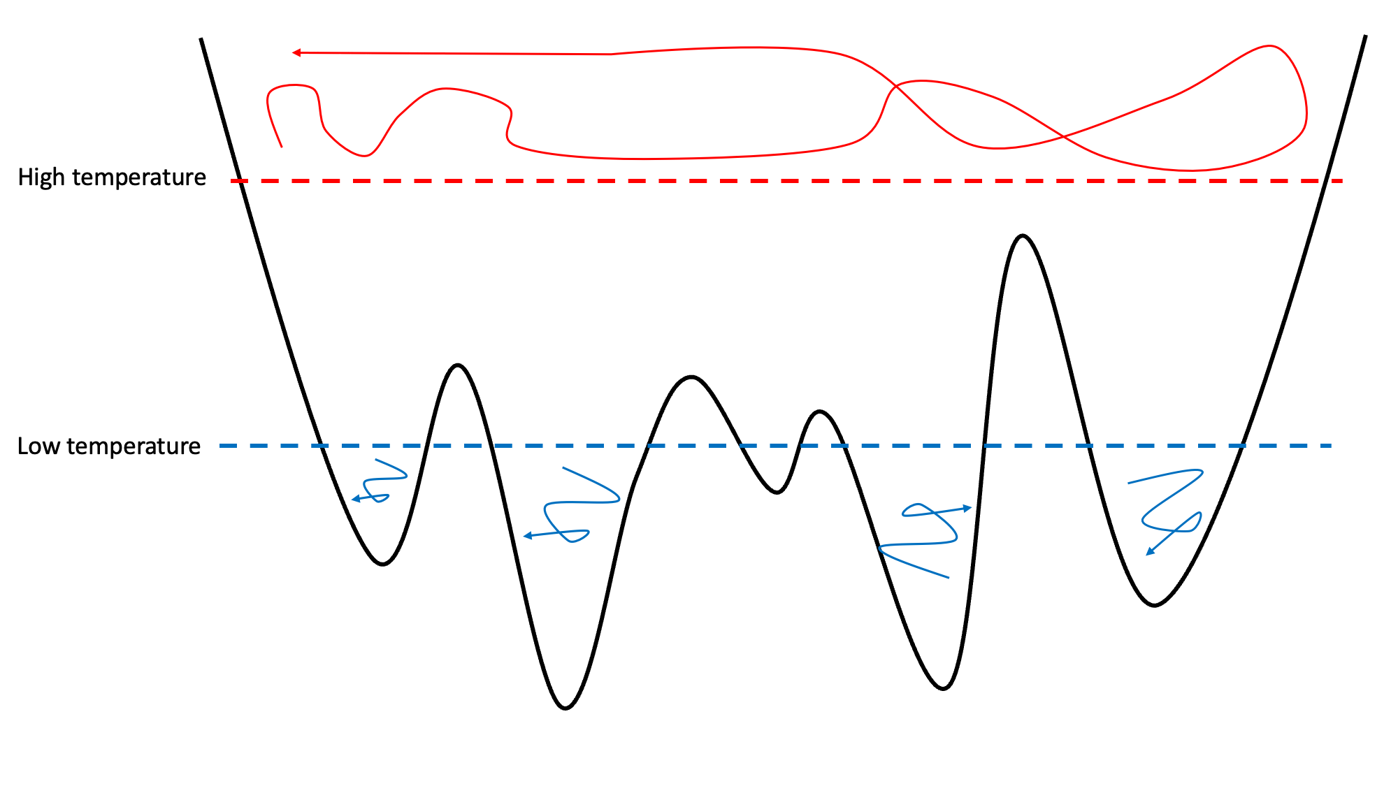
The image shows how lower temperature systems in a rough potential energy surface end up trapped in local minima. High temperature replicas can overcome the energy barriers.

The exchanges between replicas are computed using the Metropolis exchange criteria which gives the probability of accenting a swap between replicas 1 and 2:

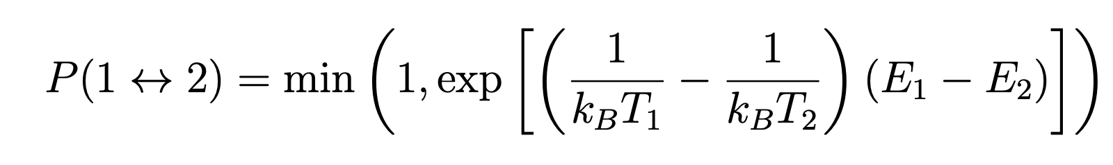
For computational efficiency, it is the temperatures that are swapped between replicas.

Example system

The code for this section can be downloaded from the git repository:

git clone --depth=1 https://www.github.com/EPCCed/archer2-advanced-use-of-lammps.git
cd exercises/3-replica-exchange-exercise

We will use a toy system: A 50 particle bead-spring polymer. This is typical of coarse-grain protein models.

The data file polymer.txt contains the system topology.

Input file

The input file run.in contains the simulation settings.

Most of the lines are general to any LAMMPS simulation. The important ones for running replica exchange are the following:

variable    T world 300.00 354.47 416.81 488.14 569.86 663.45 764.45 865.45 966.45 1000.00

and

variable    I world 0 1 2 3 4 5 6 7 8 9

Which use the world variable type to assign a temperature and corresponding index to each replica that will be run. Note here we have chosen to use 10 replicas.

fix         2 all langevin ${T} ${T} 1000 ${SEED}

The substitutions ${T} set the Langevin thermostat settings to the specified temperature for each replica.

dump        1 all atom 1000 polymer.${I}.lammpstrj

The substitution ${I} allows each replica to write its own trajectory.

temper      1000000 100 $T 2 ${SEED} ${SEED}

The temper command performs the parallel tempering run. This replaces the run command in normal LAMMPS input scripts.

The arguments are:

• Total number of timesteps to run for (1000000).
• Frequency to attempt replica swaps (every 100 timesteps).
• Temperature of this replica.
• Fix id of the thermostat (the Langevin thermostat).
• Two random number seeds, one for choosing which replicas to swap, one for the Metropolis Monte Carlo acceptance step.

Choosing the temperature scale

We have provided an input file that has 10 temperatures spanning 300K to 1000K. These have been chosen to give approximately a 30% acceptance ratio for the swap attempts. As a general rule 30% is a suitable acceptance ratio. The number of replicas needed and the temperature spacing is a function of the degrees of freedom of the system. We have used a online calculator to generate the temperature scale.

http://virtualchemistry.org/remd-temperature-generator/

Source code here: https://github.com/dspoel/remd-temperature-generator

Publication: http://dx.doi.org/10.1039/b716554d

Using:

• number of proteins = 50
• number of water = 0
• lower temperature = 300
• higher temperature = 1000
• exchange probability = 0.3

you should get the same temperature scale.

Running the simulation

To run the simulation the -partition argument must be used when running LAMMPS.

In this example we have 10 replicas so 10 partitions must be used. An example command to do this is:

mpirun -np 10 lmp -in run.in -partition 10x1

This will use 10 MPI processes to run 10 replicas of the simulation (1 MPI processes per replica).

More MPI processes per replica can be used, for example

mpirun -np 20 lmp -in run.in -partition 10x2

will run the same parallel tempering simulation but use 2 MPI processes per replica.

For this toy example of only 50 atoms there will be no parallel speedup from doing this.

Note

On ARCHER2 the provided batch script run.slurm will run this on the compute nodes. Remember that ARCHER2 does not have mpirun and the only way to run MPI programs is with srun on the compute nodes.

sbatch run.slurm

Simulation output

The master log file log.lammps contains the information about which temperature each replica is at each timestep. Below is an example:

LAMMPS (29 Sep 2021)
Running on 10 partitions of processors
Setting up tempering ...
Step T0 T1 T2 T3 T4 T5 T6 T7 T8 T9
0 0 1 2 3 4 5 6 7 8 9
100 1 0 3 2 5 4 7 6 9 8
200 1 0 3 2 4 5 6 7 8 9
300 2 0 3 1 4 5 6 7 8 9
400 3 1 2 0 5 4 7 6 9 8
500 3 2 1 0 5 4 8 6 9 7
600 4 2 1 0 6 3 7 5 9 8
700 3 1 2 0 6 4 7 5 9 8
800 3 2 1 0 5 4 8 6 9 7
900 4 2 1 0 6 3 7 5 9 8
1000 4 1 2 0 6 3 7 5 9 8

If we look at step 1000 we see that replica 0 has temperature index 4 (569.86 K), replica 2 has temperature index 1 (354.47), etc…

Each replica has its own log file log.lammps.n which contains the thermo output. The screen.n files contain what would usually be printed to the terminal for a normal non-replica LAMMPS run.

The files polymer.n.lammpstrj contain the trajectories of each replica. These are continuous in coordinate space, not in temperature. The temperature of each trajectory varies corresponding to the swaps listed in the master log file. Before analysis the trajectories must be re-ordered into trajectories of the same temperature.

Checking the simulation

It is important to check that parallel tempering simulations are running correctly.

Acceptance ratios

The key quantity is the acceptance ratio which is the probability of a successful swap between replicas. The number should be in the range 20 to 40 % for optimal sampling. When we setup the temperate scale we aimed for an acceptance ratio of 30%. We have provided a python script to calculate the acceptance ratio of the simulation.

module load cray-python
python acceptance_ratio.py

Output:

T indexes, Acceptance ratio
0 - 1, 0.275972402759724
1 - 2, 0.32836716328367166
2 - 3, 0.35176482351764826
3 - 4, 0.3711628837116288
4 - 5, 0.38036196380361964
5 - 6, 0.45835416458354167
6 - 7, 0.5427457254274572
7 - 8, 0.6203379662033797
8 - 9, 0.8687131286871312

We see that the lower T index have a ratio close to 0.3 which is ideal, the higher ones have a larger ratio, this is an artefact of our small toy system – The calculator we used to generate the temperature scale is designed for larger explicit solvent bio-molecular systems in the NPT ensemble.

If the ratios were too low (less than 20%) you would want to reduce the temperature differences, and use more replicas, If too high (greater than 50%) you would want to increase the temperature difference and use less replicas.

Traversal of the temperatures

It is also important to check that the replicas are fully traversing temperature space. If you plot the columns of the master log file you will see how the temperature index varies with the timestep.

module load gnuplot
gnuplot
gnuplot> plot "log.lammps" using 1:2 with lines

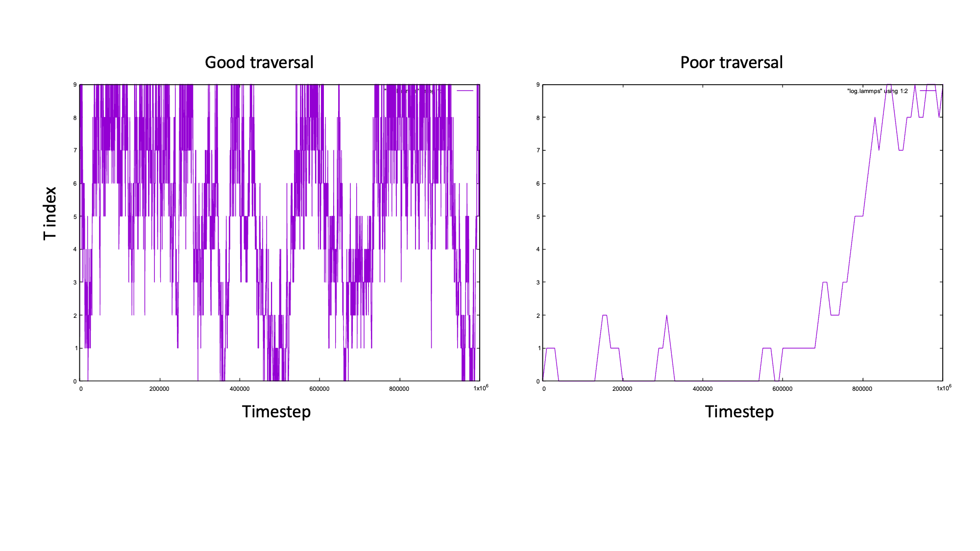
The plot on the left shows good traversal, the replica reaches T0 and T9 multiple times.

The plot on the right is an example of poor traversal (we changed the swap frequency to 10000).

Reordering the trajectories into constant temperature

This can be done using the provided python script reorder.py

python reorder.py polymer 10

Where the first argument is the prefix of the trajectory files and the second is the number of replicas.

This will produce the reordered trajectories named polymer.Tn.lammpstrj where Tn is the temperature index, i.e T0 is the first temperature (300K ), and T1 is the second temperature (354.47K) etc.

Analysing the constant temperature trajectories

We can now analyse the reordered trajectories. This can be done using the rerun command. If you move into the rerun folder you will find the input script rerun.in.

cd rerun

If you open it you will see some differences to the run script run.in. The key parts are that the data file must still be read in. The pair and bond styles are still defined the same way. The NVE and Langevin fixes are not needed as no integration is performed for a rerun. We define a compute for the analysis we want to do

compute       RG all gyration

which computes the radius of gyration of the polymer.

We then use ave/histo fix which creates a histogram of the RG values over the whole simulation and saves it to a file.

fix 4 all ave/histo 1000 1000 1000000 7 20 100 c_RG file RG_histogram_T${I}.txt start 100000

Finally the rerun command

rerun ../polymer.T${I}.lammpstrj dump x y z

This reads the re-ordered trajectories from the simulation and computes the radius of gyration for each frame.

To run this for all temperatures at once we can use the LAMMPS partition switch again.

mpirun -np 10 lmp -in rerun.in -partition 10x1

For ARCHER2 the slurm script rerun.slurm is provided.

sbatch rerun.slurm

Note that this can be done in serial individually for each temperature. It is trivially parallel as no communication is needed between the replicas we are rerunning (unlike the parallel tempering run). To do this you would just need to change the line

variable I world 0 1 2 3 4 5 6 7 8 9

to the single temperature index of interest. E.g.

variable I index 0

And then run as normal

lmp -in rerun.in

We now have the RG histograms for each temperature RG_histogram_Tn.txt.

They can be plotted using the provided gnuplot script

gnuplot -p plot.gp

On ARCHER2 remember to load the gnuplot module (if you haven’t yet)

module load gnuplot

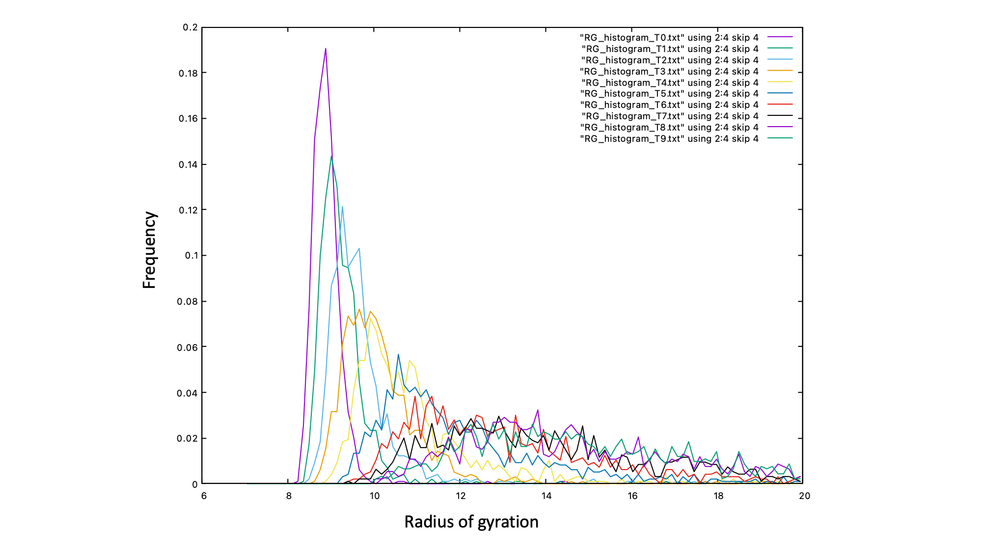
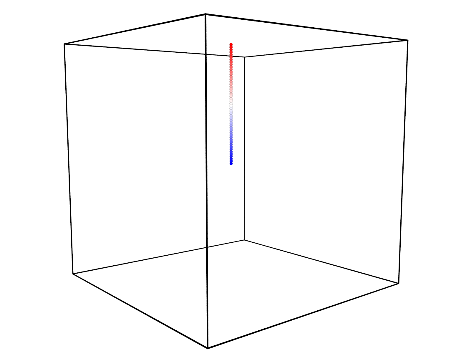
We can see that temperature index 0 (300K) has the most well defined peak with the smallest radius of gyration. This typical of a globule like polymer state. The highest temperature index 9 (1000K) has a different profile, typical of a coil like polymer state.

To reduce the noise on the histograms you would need to run the simulation longer, we have kept it short here for demonstration purposes.

The plot shows the enhanced sampling capabilities of parallel tempering. The extended high T configurations enable a greater exploration of the compact low T configurations.

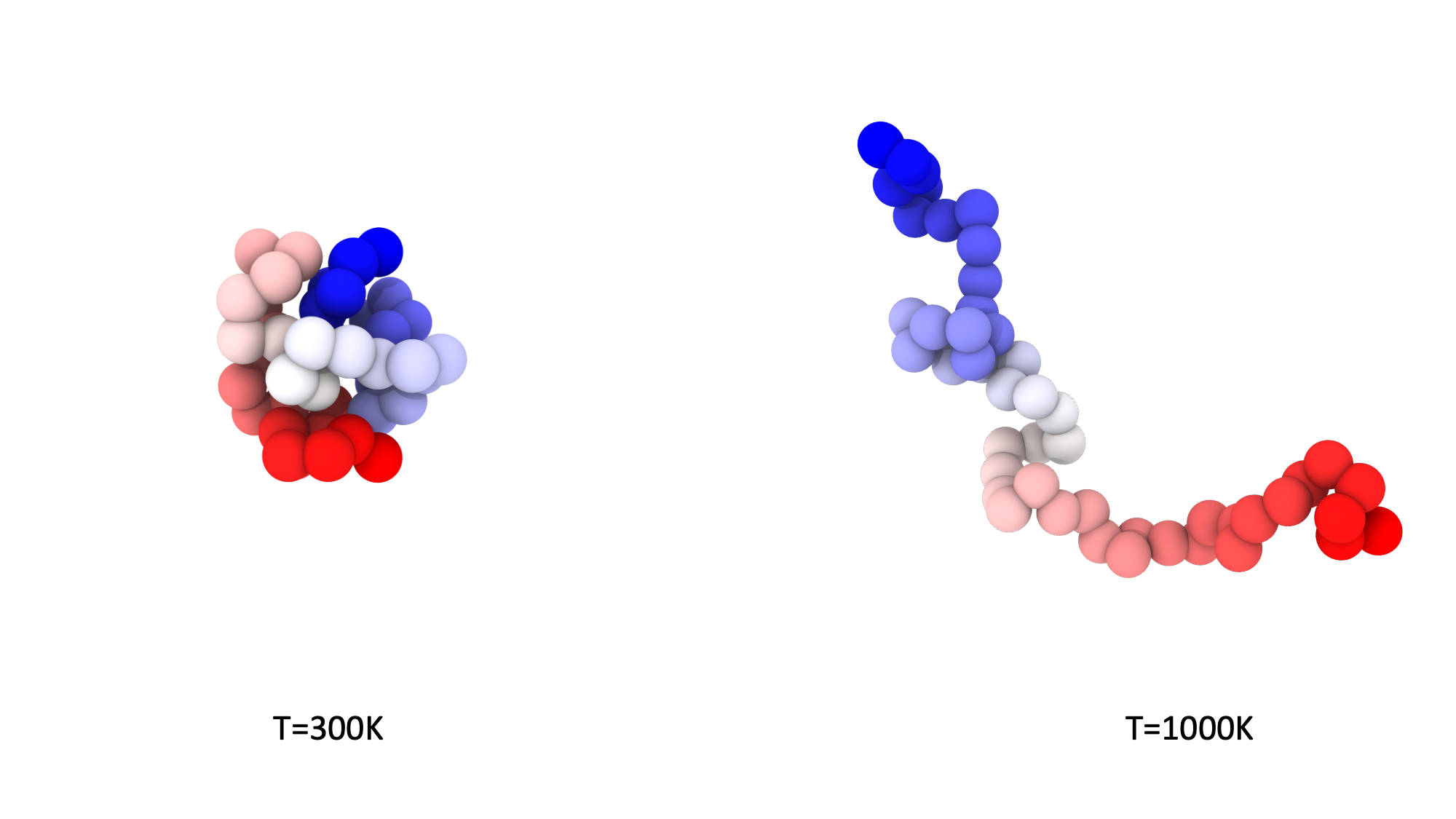
The low and high temperature configurations of the polymer are shown in the image.

Further reading

• https://docs.lammps.org/Howto_replica.html
• Parallel tempering: Theory, applications, and new perspectives http://dx.doi.org/10.1039/B509983H
• A temperature predictor for parallel tempering simulations http://dx.doi.org/10.1039/B716554D

Key Points

• Choose the temperature scale carefully.

• Check the acceptance ratios and replica traversal.

• Make sure you reorder the trajectories before analysing.