Measuring and improving LAMMPS performance
Overview
Teaching: 20 min
Exercises: 30 minQuestions
How can we run LAMMPS on ARCHER2?
How can we improve the performance of LAMMPS?
Objectives
Gain an overview of submitting and running jobs on the ARCHER2 service.
Gain an overview of methods to improve the performance of LAMMPS.
What is LAMMPS?
LAMMPS (Large-scale Atomic/Molecular Massively Parallel Simulator) is a versatile classical molecular dynamics software package, developed by Sandia National Laboratories and by its wide user-base.
It can be downloaded directly from the Sandia website.
Everything we are covering today (and a lot of other info) can be found in the LAMMPS User Manual.
Running LAMMPS on ARCHER2
ARCHER2 uses a module system. In general, you can run LAMMPS on ARCHER2 by using the LAMMPS module:
ta132ra@ln01:~> module avail lammps

------------------------ /work/y07/shared/archer2-lmod/apps/core ------------------------
   lammps-python/15Dec2023    lammps/15Dec2023    lammps/17Feb2023 (D)

  Where:
   D:  Default Module
[...]
For this course, we will be using the most recent version of the LAMMPS module (15Dec2023), not the default one.
Running module load lammps/15Dec2023 will set up your environment to use the correct LAMMPS version.
The build instructions for this version are described in the next section of the course.
Once your environment is set up, you will have access to the lmp LAMMPS executable.
Note that you will only be able to run this on a single core on the ARCHER2 login node, unless you use the slurm scheduler.
Submitting a job to the compute nodes
To run LAMMPS on multiple cores/nodes, you will need to submit a job to the ARCHER2 compute nodes.
The compute nodes do not have access to the landing home file-system – this file system is to store useful/important information.
On ARCHER2, when submitting jobs to the compute nodes, make sure that you are in your /work/ta132/ta132/<username> directory.
For this course, we have prepared a number of exercises.
You can get a copy of these exercises by running (make sure to run this from /work):
git clone --depth=1 https://www.github.com/EPCCed/archer2-advanced-use-of-lammps.git
Once this is downloaded, please cd exercises/1-performance-exercise/.
In this directory you will find three files:
run.slurmis a Slurm submission script – this will let you submit jobs to the compute nodes. Initially, it will run a single core job, but we will be editing it to run on more cores.in.ethanolis the LAMMPS input script that we will be using for this exercise. This script is meant to run a small simulation of 125 ethanol molecules in a periodic box.data.ethanolis a LAMMPS data file for a single ethanol molecule. This template will be copied by thein.lammpsfile to generate our simulation box.
Why ethanol?
The
in.ethanolLAMMPS input that we are using for this exercise is an easily edited benchmark script used within EPCC to test system performance. The intention of this script is to be easy to edit and alter when running on very varied core/node counts. By editing theX_LENGTH,Y_LENGTH, andZ_LENGTHvariables, you can increase the box size substantially. As to the choice of molecule, we wanted something small and with partial charges – ethanol seemed to fit both of those.
To submit your first job on ARCHER2, please run:
sbatch run.slurm
You can check the progress of your job by running squeue -u ${USER}. Your job state will go from PD (pending) to R (running) to CG (cancelling).
Once your job is complete, it will have produced a file called slurm-####.out – this file contains the STDOUT and STDERR produced by your job.
The job will also produce a LAMMPS log file log.out.
In this file, you will find all of the thermodynamic outputs that were specified in the LAMMPS thermo_style, as well as some very useful performance information!
After every run is complete, LAMMPS outputs a series of information that can be used to better understand the behaviour of your job.
Loop time of 197.21 on 1 procs for 10000 steps with 1350 atoms

Performance: 4.381 ns/day, 5.478 hours/ns, 50.707 timesteps/s
100.0% CPU use with 1 MPI tasks x 1 OpenMP threads

MPI task timing breakdown:
Section |  min time  |  avg time  |  max time  |%varavg| %total
---------------------------------------------------------------
Pair    | 68.063     | 68.063     | 68.063     |   0.0 | 34.51
Bond    | 5.0557     | 5.0557     | 5.0557     |   0.0 |  2.56
Kspace  | 5.469      | 5.469      | 5.469      |   0.0 |  2.77
Neigh   | 115.22     | 115.22     | 115.22     |   0.0 | 58.43
Comm    | 1.4039     | 1.4039     | 1.4039     |   0.0 |  0.71
Output  | 0.00034833 | 0.00034833 | 0.00034833 |   0.0 |  0.00
Modify  | 1.8581     | 1.8581     | 1.8581     |   0.0 |  0.94
Other   |            | 0.139      |            |       |  0.07

Nlocal:        1350.00 ave        1350 max        1350 min
Histogram: 1 0 0 0 0 0 0 0 0 0
Nghost:        10250.0 ave       10250 max       10250 min
Histogram: 1 0 0 0 0 0 0 0 0 0
Neighs:        528562.0 ave      528562 max      528562 min
Histogram: 1 0 0 0 0 0 0 0 0 0

Total # of neighbors = 528562
Ave neighs/atom = 391.52741
Ave special neighs/atom = 7.3333333
Neighbor list builds = 10000
Dangerous builds not checked
Total wall time: 0:05:34
The ultimate aim is always to get your simulation to run in a sensible amount of time. This often simply means trying to optimise the final value (“Total wall time”), though some people care more about optimising efficiency (wall time multiplied by core count). In this lesson, we will be focusing on what we can do to improve these.
Increasing computational resources
The first approach that most people take to increase the speed of their simulations is to increase the computational resources. If your system can accommodate this, doing this can sometimes lead to “easy” improvements. However, this usually comes at an increased cost (if running on a system for which compute is charged) and does not always lead to the desired results.
In your first run, LAMMPS was run on a single core.
For a large enough system, increasing the number of cores used should reduce the total run time.
In your run.slurm file, you can edit the line:
#SBATCH --tasks-per-node=1
to run on more cores. An ARCHER2 node has 128 cores, so you could potential run on up to 128 cores.
Quick benchmark
As a first exercise, fill in the table below.
Number of cores Walltime Performance (ns/day) 1 2 4 8 16 32 64 128 Do you spot anything unusual in these run times? If so, can you explain this strange result?
Solution
The simulation takes almost the same amount of time when running on a single core as when running on two cores. A more detailed look into the
in.ethanolfile will reveal that this is because the simulation box is not uniformly packed.
Note
Here are only considering MPI parallelisation – LAMMPS offers the option to run using joint MPI+OpenMP (more on that later), but for the exercises in this lesson, we will only be considering MPI.
Domain decomposition
In the previous exercise, you will (hopefully) have noticed that, while the simulation run time decreases overall as the core count is increased, the run time was the same when run on one processor as it was when run on two processors. This unexpected behaviour (for a truly strong-scaling system, you would expect the simulation to run twice as fast on two cores as it does on a single core) can be explained by looking at our starting simulation configuration and understanding how LAMMPS handles domain decomposition.
In parallel computing, domain decomposition describes the methods used to split calculations across the cores being used by the simulation. How domain decomposition is handled varies from problem to problem. In the field of molecular dynamics (and, by extension, within LAMMPS), this decomposition is done through spatial decomposition – the simulation box is split up into a number of blocks, with each block being assigned to their own core.
By default, LAMMPS will split the simulation box into a number of equally sized blocks and assign one core per block. The amount of work that a given core needs to do is directly linked to the number of atoms within its part of the domain. If a system is of uniform density (i.e., if each block contains roughly the same number of particles), then each core will do roughly the same amount of work and will take roughly the same amount of time to calculate interactions and move their part of the system forward to the next timestep. If, however, your system is not evenly distributed, then you run the risk of having a number of cores doing all of the work while the rest sit idle.
The system we have been simulating looks like this at the start of the simulation:
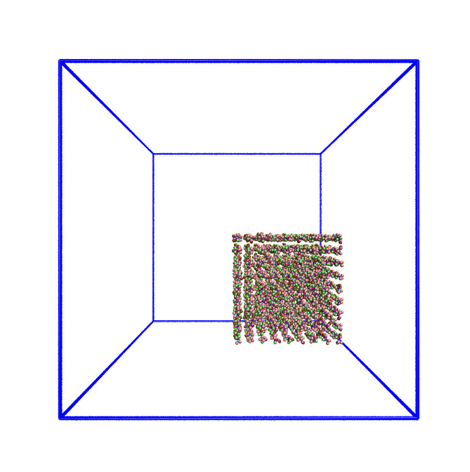
As this is a system of non-uniform density, the default domain decomposition will not produce the desired results.
LAMMPS offers a number of methods to distribute the tasks more evenly across the processors.
If you expect the distribution of atoms within your simulation to remain constant throughout the simulation, you can use a balance command to run a one-off re-balancing of the simulation across the cores at the start of your simulation.
On the other hand, if you expect the number of atoms per region of your system to fluctuate (e.g. as is common in evaporation), you may wish to consider recalculating the domain decomposition every few timesteps with the dynamic fix balance command.
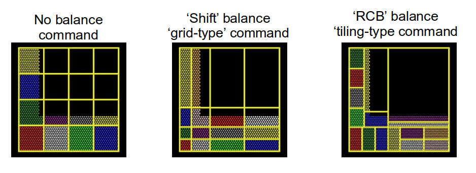
For both the static, one-off balance and the dynamic fix balance commands, LAMMPS offers two methods of load balancing – the “grid-like” shift method and the “tiled” rcb method.
The diagram below helps to illustrate how these work.
Using better domain decomposition
In your
in.ethanolfile, uncomment thefix balancecommand and rerun your simulations. What do you notice about the runtimes? We are using the dynamic load balancing command – would the static, one-offbalancecommand be effective here?Solution
The runtimes decrease significantly when running with dynamic load balancing. In this case, static load balancing would not work as the ethanol is still expanding to fill the simulation box. Once the ethanol is evenly distributed within the box, you can remove the dynamic load balancing.
Playing around with dynamic load balancing
In the example, the
fix balanceis set to be recalculated every 1,000 timesteps. How does the runtime vary as you change this value? I would recommend trying 10, 100, and 10,000.Solution
The simulation time can vary drastically depending on how often re-balancing is carried out. When using dynamic re-balancing, there is an important trade-off between the time gained from re-balancing and the cost involved with recalculating the load balance among cores.
You can find more information about how LAMMPS handles domain decomposition in the LAMMPS manual balance and fix balance sections.
Considering neighbour lists
Let’s take another look at the profiling information provided by LAMMPS:
Section |  min time  |  avg time  |  max time  |%varavg| %total
---------------------------------------------------------------
Pair    | 68.063     | 68.063     | 68.063     |   0.0 | 34.51
Bond    | 5.0557     | 5.0557     | 5.0557     |   0.0 |  2.56
Kspace  | 5.469      | 5.469      | 5.469      |   0.0 |  2.77
Neigh   | 115.22     | 115.22     | 115.22     |   0.0 | 58.43
Comm    | 1.4039     | 1.4039     | 1.4039     |   0.0 |  0.71
Output  | 0.00034833 | 0.00034833 | 0.00034833 |   0.0 |  0.00
Modify  | 1.8581     | 1.8581     | 1.8581     |   0.0 |  0.94
Other   |            | 0.139      |            |       |  0.07
There are 8 possible MPI tasks in this breakdown:
Pairrefers to non-bonded force computations.Bondincludes all bonded interactions, (so angles, dihedrals, and impropers).Kspacerelates to long-range interactions (Ewald, PPPM or MSM).Neighis the construction of neighbour lists.Commis inter-processor communication (AKA, parallelisation overhead).Outputis the writing of files (log and dump files).Modifyis the fixes and computes invoked by fixes.Otheris everything else.
Each category shows a breakdown of the least, average, and most amount of wall
time any processor spent on each category – large variability in this
(calculated as %varavg) indicates a load imbalance (which can be caused by the
atom distribution between processors not being optimal). The final column,
%total, is the percentage of the loop time spent in the category.
A rule-of-thumb for %total on each category
Pair: as much as possible.Neigh: 10% to 30%.Kspace: 10% to 30%.Comm: as little as possible. If it’s growing large, it’s a clear sign that too many computational resources are being assigned to a simulation.
In the example above, we notice that the majority of the time is spent in the Neigh section – e.g. a lot of time is spent calculating neighbour lists.
Neighbour lists are a common method for speeding up simulations with short-ranged particle-particle interactions.
Most interactions are based on inter-particle distance and traditionally the distance between every particle and every other particle would need to be calculated every timestep (this is an O(N²) calculation!).
Neighbour lists are a way to reduce this to an ~O(N) calculation for truncated short-ranged interactions.
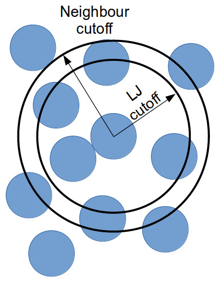
Instead of considering all interactions between every particle in a system, you can generate a list of all particles within the truncation cutoff plus a little bit more.
Depending on the size of that “little bit more” and the details of your system, you can work out how quickly a particle that is not in this list can move to be within the short-ranged interaction cutoff.
With this time, you can work out how frequently you need to update this list.
Doing this reduces the number of times that all inter-particle distances need to be calculated: every few timestep, the inter-particle distances for all particle pairs are calculated to generate the neighbour list for each particle; and in the interim, only the inter-particle distances for particles within a neighbour list need be calculated (as this is a much smaller proportion of the full system, this greatly reduces the total number of calculations).
If we dig a bit deeper into our in.ethanol LAMMPS input file, we will notice the following lines:
variable        NEIGH_TIME  equal      1    # neigh_modify every x dt
...
neigh_modify    delay 0 every ${NEIGH_TIME} check no
These lines together indicate that LAMMPS is being instructed to rebuild the full neighbour list every timestep (so this is not a very good use of neighbour lists).
Changing neighbour list update frequency
Change the
NEIGH_TIMEvariable to equal 10. How does this affect the simulation runtime?Now change the
NEIGH_TIMEvariable to equal 1000. What happens now?
Neighbour lists only give physical solutions when the update time is less than the time it would take for a particle outwith the neighbour cutoff to get to within the short-ranged interaction cutoff. If this happens, the results generated by the simulation become questionable at best and, in the worst case, LAMMPS will crash.
You can estimate the frequency at which you need to rebuild neighbour lists by running a quick simulation with neighbour list rebuilds every timestep:
neigh_modify delay 0 every 1 check yes
and looking at the resultant LAMMPS neighbour list information in the log file generated by that run.
Total # of neighbors = 1313528
Ave neighs/atom = 200.20241
Ave special neighs/atom = 7.3333333
Neighbor list builds = 533
Dangerous builds = 0
The Neighbor list builds tells you how often neighbour lists needed to be rebuilt.
If you know how many timesteps your short simulation ran for, you can estimate the frequency at which you need to calculate neighbour lists by working out how many steps there are per rebuild on average.
Provided that your update frequency is less than or equal to that, you should see a speed up.
In this section, we only considered changing the frequency of updating neighbour lists.
Two other factors that contribute to the time taken to calculate neighbour lists are the pair_style cutoff distance and the neighbor skin distance.
Decreasing either of these will reduce the number of particles within the neighbour cutoff distance, thereby decreasing the number of interactions being calculated each timestep.
However, decreasing these will mean that lists need to be rebuilt more frequently – it’s always a fine balance.
You can find more information in the LAMMPS manual about neighbour lists and the neigh_modify command.
Some further tips
Fixing bonds and angles
A lot of interesting systems involve simulating particles bonded into molecules. In a lot of classical atomistic systems, some of these bonds fluctuate significantly and at high frequencies, while not causing much interesting physics (think e.g. carbon-hydrogen bonds in a hydrocarbon chain). As the timestep is restricted by the fastest-moving part of a simulation, the frequency of fluctuation of these bonds restricts the length of the timestep that can be used in the simulation. Using longer timesteps results in longer “real time” effects being simulated for the same amount of compute power, so being restricted to a shorter timestep because of “boring” bonds can be frustrating.
LAMMPS offers two methods of restricting these bonds (and their associated angles):
the SHAKE and RATTLE fixes.
Using these fixes will ensure that the desired bonds and angles are reset to their equilibrium length every timestep.
An additional constraint is applied to these atoms to ensure that they can still move while keeping the bonds and angles as specified.
This is especially useful for simulating fast-moving bonds at higher timesteps.
You can find more information about this in the LAMMPS manual
Hybrid MPI+OpenMP runs
When looking at the LAMMPS profiling information, we briefly mentioned that the proportion of time spent calculating Kspace should fall within the 10-30% region.
Kspace can often come to dominate the time profile when running with a large number of MPI ranks.
This is a result of the way that LAMMPS handles the decomposition of k-space across multiple MPI ranks.
One way to overcome this problem is to run your simulation using hybrid MPI+OpenMP.
To do this, you must ensure that you have compiled LAMMPS with the OMP package.
On ARCHER2, you can edit the run.slurm file that you have been using to include the following:
#SBATCH --tasks-per-node=64
#SBATCH --cpus-per-task=2

[...]

export OMP_NUM_THREADS=2
export SRUN_CPUS_PER_TASK=$SLURM_CPUS_PER_TASK

srun lmp -sf omp -i in.ethanol -l ${OMP_NUM_THREADS}_log.out
Setting the variable OMP_NUM_THREADS will let LAMMPS know how many OpenMP threads will be used in the simulation.
Setting --tasks-per-node and --cpus-per-task will ensure that Slurm assigns the correct number of MPI ranks and OpenMP threads to the executable.
Setting the LAMMPS --sf omp flag will result in LAMMPS using the OMP version of any command in your LAMMPS input script.
Running hybrid jobs efficiently can add a layer of complications, and a number of additional considerations must be taken into account to ensure the desired results. Some of these are:
- The product of the values assigned to
--tasks-per-nodeand--cpus-per-taskshould be less than or equal to the number of cores on a node (on ARCHER2, that number is 128 cores). - You should try to restrict the number of OpenMP threads per MPI task to fit on a single socket. For ARCHER2, the sockets (processors) are so large that they have been subdivided into a number of NUMA regions. Each ARCHER2 node 2 sockets, each socket has 4 NUMA regions, each of which has 16 cores, for a total of 8 NUMA regions per node. Therefore, for an efficient LAMMPS run, you would not want to use more than 16 OpenMP processes per MPI task.
-
In a similar vein to the above, you also want to make sure that your OpenMP threads are kept within a single NUMA region. Spanning across multiple NUMA regions will decrease the performance (significantly).
These are only some of the things to bear in mind when considering using hybrid MPI+OpenMP to speed up k-space calculations.
Using
verlet/splitinsteadAnother way to decrease the amount of compute being used by k-space calculations is to use the
run_style verlet/splitcommand. This lets you split your force calculations across two partitions of cores. Using this would let you define the partitions (and the amount of computational resources assigned to this partition) on which long-ranged k-space interactions are calculated.You can find out more about this in the LAMMPS manual
Key Points
LAMMPS offers a number of built in methods to improve performance.
It is important to spend some time understanding your system and considering its performance.
Where possible, always run a quick benchmark of your system before setting up a large run.