Running GROMACS simulations on ARCHER2

Overview

Teaching: 25 min
Exercises: 20 min

Questions

• How do I run a simulation with GROMACS?

• How can I equilibrate my system?

Objectives

• Understand what GROMACS does under the hood.

• Learn about GROMACS MDP files.

• Run a GROMACS simulation on the ARCHER2 compute nodes.

What is classical molecular dynamics

So far in this course, we have been preparing a system that we would like to simulate with GROMACS. We have seen how to take a .pdb file from the protein database and prepare it using some GROMACS tools. We’ve also seen how to assign a forcefield for our simulation. Now that our system is ready, how do we run a simulation of our system using GROMACS? Before we look into this, let’s consider what is means to run a simulation in GROMACS.

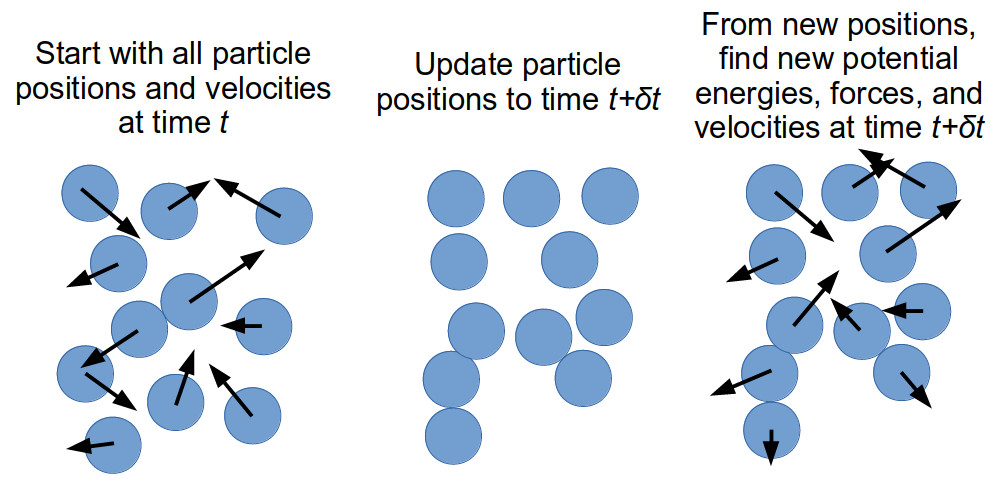
GROMACS is a classical molecular dynamics solver. Classical molecular dynamics is a method of simulating the interactions and resultant movement of particles through time. Generally, particles will have a function defining their interactions with other particles (in our case, this is the forcefield that we used when generating the topol.top file). From these interactions, we can calculate the potential energy of the system and the force acting on each particle in the system by using the Newtonian equations of motion. We can use the current position of a particle and the force acting on it to derive the acceleration and velocity of the particle at this time. Once we have calculated the velocity of each particle, we can allow our system to go forward in time by a small increment. If the increment is small enough, we can assume that the velocity of our particles remains constant over the duration of the timestep, and can therefore determine the position of each particle in our system once the timestep is complete. From these new positions, we can calculate the potential energy, from which we derive the force, acceleration, and new velocity of each particle in our system, and with which we can bring our system forward in time by a small increment. We can keep repeating this for as long as we want.

The repetitive nature of classical molecular dynamics makes it very suitable for running on computers. Furthermore, since its first use in 1957, a number of methods and techniques have been developed to allow for larger systems to be simulated for longer times, as well as methods for making sure that the simulation time is spent looking at something significant and of interest. In this lesson, we will be discussing some of these methods and techniques and how to implement them in GROMACS.

Running a simulations

For this session, you will need a copy of the 5pep-neutral.gro and topol.top files generated in the previous session. You can either copy these across or use pregenerated ones. To get the pregenerated files, run:

  svn checkout https://github.com/EPCCed/20220421_GROMACS_introduction/trunk/exercises

Once this is copied, go into the exercises/running_gromacs directory. This directory contains:

• 5pep-neutral.gro – This is a copy of the solvated and ionised system you prepared in the previous session. It contains information on the particles types, particle positions, bonds, and angles.
• topol.top – This is a copy of the GROMACS topology file that you prepared in the last session. It contains information about the forcefield used for this system.
• minim.mdp and npt.mdp – These are GROMACS molecular dynamics parameter files. We will be exploring these in details during this session.
• sub_ener_minim.slurmand sub_npt.slurm – These are Slurm submission scripts. They will let you submit GROMACS simulations to the ARCHER2 compute nodes.

The GROMACS molecular dynamics parameters (MDP) file

A GROMACS molecular dynamics parameter file lets you define a number of parameters for your simulation. In this file, you can set such information as: what specific method you should use to move your simulation from timestep to timestep; how large your timestep is; how many timesteps your simulation should run for; whether (and how) to fix the temperature and/or pressure of your system; what (if any) methods you want to include to speed up running your simulation; how you want to handle long-ranged interactions; what outputs you want from your simulation and how frequently you would like those; and a lot of other things.

Energy minimisation

Before running a “useful” simulation, we will want to equilibrate our system. In the previous session, we added water and ions to our system to random positions within our simulation box. This may mean that some of their positions or orientations are not physically likely. For example when randomly adding water molecules to our simulation box, we may have ended up with a number of molecules whose oxygen atoms are close to one another, or with an ion in close proximity to a part of our protein with a similar charge. By equilibrating our system before running it, we can push our simulation towards a more physically realistic state.

There are many ways of equilibrating a system. You can:

• Run an equilibration simulation that starts at a temperature of 0 K and increases slowly to the temperature that you’re wanting to simulate;
• Run an equilibration simulation with a very small timestep to allow your system to “relax” into a more realistic configuration
• Reduce the potential energy of a system by using an energy-minimisation techniques;
• etc.

GROMACS handily provides a number of energy minimisation protocols so we shall use one of these. The protocol we will use if the “steepest descent” algorithm. This algorithm will effectively force our system into a potential energy minimum thereby ensuring that our system is “relaxed”. If you want to find out more about the way this works, the gradient descent Wikipedia page is a great starting place.

  ; minim.mdp - taken from http://www.mdtutorials.com/gmx/
  ; Parameters describing what to do, when to stop and what to save
  integrator      = steep     ; steepest descent algorithm
  emtol           = 1000.0    ; Stop minimization when max. force < 1000.0 kJ/mol/nm
  emstep          = 0.01      ; Minimization step size
  nsteps          = 50000     ; Maximum number of (minimization) steps to perform

  ; Logs and outputs
  nstlog          = 500       ; number of steps between each log output
  nstenergy       = 500       ; number of steps between each energy file output
  nstxout         = 500       ; number of steps between each output to the coordinate file
  
  ; Parameters describing how to find the neighbors of each atom and how to calculate the interactions
  nstlist         = 1         ; Frequency to update the neighbor list and long range forces
  cutoff-scheme   = Verlet    ; Buffered neighbor searching
  ns_type         = grid      ; Method to determine neighbor list (simple, grid)
  coulombtype     = PME       ; Treatment of long range electrostatic interactions
  rcoulomb        = 1.0       ; Short-range electrostatic cut-off
  rvdw            = 1.0       ; Short-range Van der Waals cut-off
  pbc             = xyz       ; Periodic Boundary Conditions in all 3 dimensions

Before we can run this, we will use the GROMACS pre-processing tool grompp to group all of the information for our simulation into a simulation input file (what GROMACS calls a “portable binary file” or .tpr file). We can do this from the ARCHER2 login node by running:

  gmx grompp -f minim.mdp -c 5pep-neutral.gro -p topol.top -o ener_minim.tpr

This will generate our simulation run file ener_minim.tpr. We can now use this to run a GROMACS simulation on ARCHER2. We could run this on the ARCHER2 login node but that would take much too long and use up valuable shared resources. Instead, we will submit a job to the Slurm scheduler and have this run on the compute nodes. There, we will be able to use the full 128 cores on the nodes and ensure that our job will finish more quickly.

To submit your job on the login nodes, run:

  sbatch sub_ener_minim.slurm

If we take a look at the Slurm submission script, we will notice that there are a number of commands defining what resources we want to reserve with Slurm (all of the commands that start with #SBATCH), a command to load the GROMACS module that we’ve been using, a command to define the number of OpenMP threads we want (we will talk more about this in the final session of today when we discuss performance), and a GROMACS command line (it is commented with a # below to ensure that no-one accidentally copies it to run on the ARCHER2 login nodes):

  # gmx mdrun -ntomp ${SLURM_CPUS_PER_TASK} -v -s ener_minim.tpr

The mdrun command indicates that this is a molecular dynamics run – though the aim of this is to equilibrate the system, this still constitutes a GROMACS molecular dynamics simulation. the -v flag specifies that we would like a verbose output to the GROMACS log file – this can be particularly useful for debugging your simulation when anything goes wrong. The -s flag lets us define our GROMACS .tpr file. Finally, the -ntomp flag defines the number of OpenMP threads we want per MPI process (in this case one).

You can check that your job is in the queue by running:

  squeue --me

Once your job has completed, you will notice that a number of outputs have been generated:

• md.log – A text file that contains all of the thermodynamic information output during the run (e.g. energy breakdowns, instantaneous pressure and temperature, system density, etc.).
• ener.edr – A binary file that contains all of the thermodynamic information output during the run (e.g. energy breakdowns, instantaneous pressure and temperature, system density, etc.).
• traj.trr – A binary that contains details of the simulation trajectory.
• confout.gro – A text file containing the particle coordinates and velocities for the final step of the simulation.
• slurm-#######.out – The Slurm output and error file for this job.

From these files, we can extract useful information to check that our jobs have completed successfully. For instance, we can use the GROMACS energy command to extract the potential energy of our system at every logged timestep and check that the energy is now sensible. We can do this by running:

  gmx energy -f ener.edr -o potential.xvg

Select option 10 to plot the total potential energy of the system and option 0 to exit the program. This will have generated a new file called potential.xvg – this is an XMGrace file that has the timestep in the first column and the total potential energy of the system in the second column. We can plot it to check that the energy has decreased and is now at or near a minimum.

NPT simulations

Now that we have equilibrated our system, we can move on to simulating it in more physical conditions. We will run a simulation in the isobaric-isothermic ensemble (fixed pressure and temperature).

For this step, we will need the topol.top and confout.gro files generated by out equilibration step. Like with energy minimisation, we will combine these along with a GROMACS molecular dynamics parameter file to create our portable binary file.

In a new directory, copy the topol.top, confout.gro, npt.mdp and sub_npt.slurm files. Then run:

  gmx grompp -f npt.mdp -c confout.gro -r confout.gro -p topol.top -o npt.tpr

The file npt.mdp has the following commands:

  ; npt.mdp -- taken from: https://docs.bioexcel.eu/gromacs_bpg/
  ; Intergrator, timestep, and total run time
  integrator               = md                ; Leap-frog MD algorithm
  dt                       = 0.002             ; Sets timestep at 2 ns
  nsteps                   = 500000            ; Sim will run 500,000 timesteps
  
  ; Logs and outputs
  nstlog                   = 500               ; Output to md.log every 500 dt
  nstenergy                = 500               ; Output to ener.edr every 500 dt
  nstxout                  = 500               ; Output to trajj.trr every 500 dt
  
  ; Bond constraints
  constraints              = h-bonds           ; Make H bonds in protein be rigid
  constraint-algorithm     = lincs             ; Define algorithm to make bonds rigid
  
  ; Van der Waals interactions
  vdwtype                  = Cut-off           ; Define type of short-ranged interaction
  rvdw                     = 1.0               ; Define short-ranged cutoff as 1 nm
  cutoff-scheme            = Verlet            ; Generate pair lists to speed up simulation
  DispCorr                 = EnerPres          ; Apply corrections to mitigate using cutoff
  pbc                      = xyz               ; PBC in all 3 dimensions
  
  ; Coulombic interactions
  coulombtype              = PME               ; Define type of long-ranged interactions
  rcoulomb                 = 1.0               ; Define long-ranged cutoff as 1nm
  
  ; Thermostat
  tcoupl                   = V-rescale         ; Define type of thermostat
  tc-grps                  = Protein  SOL NA   ; Define groups to be affected by thermostat
  ref-t                    = 300      300 300  ; Define temperature for each group in Kelvins
  tau-t                    = 0.1      0.1 0.1  ; Define temperature coupling time
  
  ; Barostat
  pcoupl                   = Parrinello-Rahman ; Define type of barostat
  ref-p                    = 1.0               ; Define system pressure in bars
  tau-p                    = 2.0               ; Define pressure coupling time
  compressibility          = 4.5e-5            ; Define compressibility of system in bar^-1

You will notice that we have not defined some of the parameters that we had defined in ener_minim.mdp. This is because, for this simulation, we are happy to use the GROMACS default values for these parameters. GROMACS will set a number of simulations parameters to a default value if they are left unspecified – if you are running something that GROMACS expects you to run (e.g. if you are running a “standard” biochemical system) you should be fine. If, however, you are running something different, your system may well produce unexpected and non-physical results unless you are careful with what defaults you allow.

As before, we will be running this on the compute nodes by using:

  sbatch sub_npt.slurm

This simulation will take around 7 minutes to complete and, once it is complete, you will have a similar set of files generated as were produced in the energy minimisation step but with one addition. There is now also a GROMACS checkpoint (.cpt) file that keeps track of information related to the barostat and thermostat. With this file, you can restart simulations while ensuring that your temperature and pressure coupling are not wrong.

Common advanced molecular dynamics techniques used

Perdiodic boundary conditions

Boundary effects can be a problem in molecular dynamics. If you are simulating just the simulation box you built, you will end up with either surface-like boundaries at the edges of your simulation box or with your simulation being surrounded by an infinity vacuum. Either of these can affect the physics of the system you are studying.

One way to get around this is to apply periodic boundary conditions (PBCs). PBCs are a method of simulating your system as if it is in bulk. These work by considering that your system is in the centre of a number of replicas of your system. When a particle from your simulation box exits through the left-hand side of your box, an identical image of this particle originating from an exact image of your simulation box will enter through the right-hand side of your box.

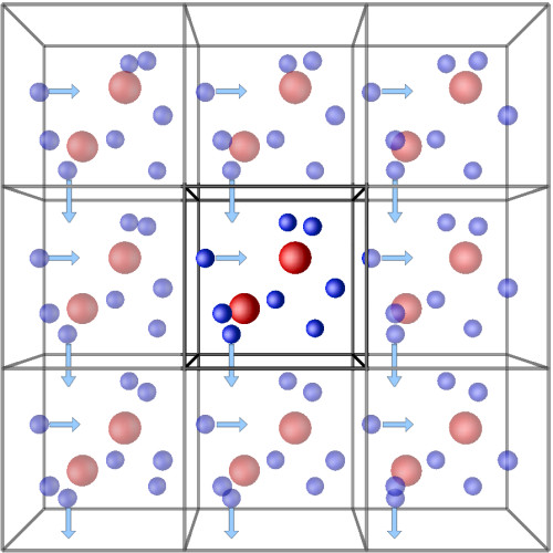
With PBCs, you are effectively simulating an infinite crystal, with your simulation box as the unit cell. This means that long-ranged (electrostatic) interactions can be solved to a high degree of accuracy by using Fourier transforms.

One must be careful when using PBCs – if your system is too small, you may end up in a situation where parts of your system are interacting with their periodic images. In that case, those parts of the system will be affecting and dictating their own behaviour! This is not correct physically.

Neighbour lists

As you have seen, each step in a molecular dynamics simulation requires you to calculate the potential energy acting on every particle in your system. Usually, simulations will use pairwise particle interactions that depend on the inter-particle distance of each particle with every other particle.

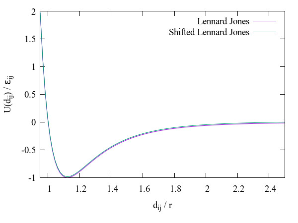
Calculating the distance between each pair of particles can be costly – this will require O(N^2) calculations per timestep! Furthermore, a lot of these pairwise interactions (such as the Lennard-Jones potential we have been using to simulate our van der Waals interactions) tend to 0 on a scale much smaller than the size of your simulation box (and are even truncated at a cutoff distance). This means that we are spending a lot of time calculating the distance between particle pairs that will effectively not be interacting.

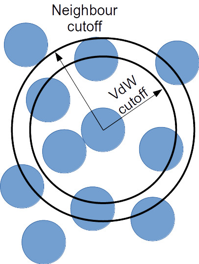
Neighbour lists allow us to be more selective and more efficient when running our simulations. If we consider a cutoff that is slightly larger than our van der Waals cutoff, we can generate for each particle a list of the other particles that fall within our cutoff. These particles are the most likely contenders to either already be within our short-ranged interaction distance or to make it into this distance for the next few timesteps. Therefore, instead of considering the inter-particle distance for all particle pairs, we can consider only the distances for particles within our neighbour list. This will reduce the runtime per timestep significantly. Furthermore, for systems at or near uniform density, this results in the expected computational time of your system to increase as ~O(N) rather than O(N^2) when you increase the number of particles of your system (e.g. doubling your system size should double your simulation time rather than quadruple it). Note that this is only true for the time spent calculating short-ranged interactions.

Key Points

• GROMACS simulation parameters are defined in a .mdp file

• GROMACS simulations are prepared using the grompp tool.

• GROMACS simulations are run using the mdrun command.