All in One View
Content from Welcome
Last updated on 2026-03-31 | Edit this page
Overview
Questions
- “What can I expect from this course?”
- “How will the course work and how will I get help?”
- “How can I give feedback to improve the course?”
Objectives
- “Understand how this course works, how I can get help and how I can give feedback.”
Course structure and method
Rather than having separate lectures and practical sessions, this course is taught following The Carpentries methodology where we all work together through material learning key skills and information throughout the course. Typically, this follows the method of the instructor demonstrating and then the attendees doing along with the instructor.
The instructors are available to assist you and to answer any questions you may have as we work through the material together. You should feel free to ask questions of the instructor whenever you like. The instructor will also provide many opportunities to pause and ask questions.
We will also make use of a shared collaborative document - the etherpad. You will find a link to this collaborative document on the course page. We will use it for a number of different purposes, for example, it may be used during exercises and instructors and helpers may put useful information or links in the etherpad that help or expand on the material being taught. If you have useful information to share with the class then please do add it to the etherpad. At the end of the course, we take a copy of the information in the etherpad, remove any personally-identifiable information, and post this on the course archive page so you should always be able to come back and find any information you found useful.
Introductions
Let’s use the etherpad to introduce ourselves. Please go to this course’s etherpad and let us know the following: - Your name - Your place of work - Whether this is your first time using ARCHER2? - Whether this is your first time using LAMMPS? - Why are you interested in learning how to use LAMMPS? - What systems are you looking to simulate?
Feedback
Feedback is integral to how we approach training both during and after the course. In particular, we use informal and structured feedback activities during the course to ensure we tailor the pace and content appropriately for the attendees, and feedback after the course to help us improve our training for the future.
You will be issued with red and green “stickies” (or shown how to use their virtual equivalent for online courses) to allow you to give the instructor and helpers quick visual feedback on how you are getting on with the pace and the content of the course. If you are comfortable with the pace/content then you should place your green sticky on the back of your laptop; if you are stuck, have questions, or are struggling with the pace/content then you should place the red sticky on the back of your laptop and a helper will come and speak to you. The instructor may also ask you to use the stickies in other, specific situations.
At the lunch break (and end of days for multi-day courses) we will also run a quick feedback activity to gauge how the course is matching onto attendees requirements. Instructors and helpers will review this feedback over lunch, or overnight, provide a summary of what we found at the start of the next session and, potentially, how the upcoming material/schedule will be changed to address the feedback.
Finally, you will be provided with the opportunity to provide feedback on the course after it has finished. We welcome all this feedback, both good and bad, as this information in key to allow us to continually improve the training we offer.
- “The course will be flexible to best meet the learning needs of the attendees.”
- “Feedback is an essential part of our training to allow us to continue to improve and make sure the course is as useful as possible to attendees.”
Content from Connecting to ARCHER2 and transferring data
Last updated on 2026-03-31 | Edit this page
Overview
Questions
- “How can I access ARCHER2 interactively?”
Objectives
- “Understand how to connect to ARCHER2.”
Purpose
Attendees of this course will get access to the ARCHER2 HPC facility. You will have the ability to request an account and to login to ARCHER2 before the course begins. In this session, we will talk you through getting access to ARCHER2. Please be aware that you will need to follow the ARCHER2 Code of Conduct as a condition for access.
Note that if you are not able to login to ARCHER2 and do not attend this session, you may struggle to run the course exercises as these were designed to run on ARCHER2 specifically.
Connecting using SSH
The ARCHER2 login address is
login.archer2.ac.ukTo login using ssh, use the command:
Access to ARCHER2 is via SSH using both a password and a passphrase-protected SSH key pair.
Passwords and password policy
When you first get an ARCHER2 account, you will get a single-use password from the SAFE which you will be asked to change to a password of your choice. Your chosen password must have the required complexity as specified in the ARCHER2 Password Policy.
The password policy has been chosen to allow users to use both
complex, shorter passwords and long, but comparatively simple passwords.
For example, passwords in the style of both LA10!£lsty and
correcthorsebatterystaple would be supported.
SSH keys
As well as password access, users are required to add the public part of an SSH key pair to access ARCHER2. The public part of the key pair is associated with your account using the SAFE web interface. See the ARCHER2 User and Best Practice Guide for information on how to create SSH key pairs and associate them with your account:
MFA/TOTP
Multi-factor authentication, under the form of timed one-time passwords, are now mandatory on ARCHER2 accounts. To create one, please follow the instructions in our SAFE documentation.
Data transfer services: scp, rsync
ARCHER2 supports a number of different data transfer mechanisms. The one you choose depends on the amount and structure of the data you want to transfer and where you want to transfer the data to. The two main options are:
-
scp: The standard way to transfer small to medium amounts of data off ARCHER2 to any other location -
rsync: Used if you need to keep small to medium data-sets synchronised between two different locations
More information on data transfer mechanisms can be found in the ARCHER2 User and Best Practice Guide:
- “ARCHER2’s login address is
login.archer2.ac.uk.”
Content from An introduction to LAMMPS on ARCHER2
Last updated on 2026-03-31 | Edit this page
Overview
Questions
- “What is LAMMPS?”
- “How do I run jobs in ARCHER2?”
Objectives
- “Understand what LAMMPS is.”
- “Learn how to launch jobs on ARCHER2 using the slurm batch system.”
- “Run a LAMMPS benchmark exercise to see how benchmarking can help improve code performance.”
ARCHER2 system overview
Architecture
The ARCHER2 HPE Cray EX system consists of a number of different node types. The ones visible to users are:
- Login nodes
- Compute nodes
- Data analysis (pre-/post- processing) nodes
All of the non-GPU node types have the same processors: AMD EPYCTM 7742, 2.25GHz, 64-cores. All non-GPU nodes are dual socket nodes so there are 128 cores per node.
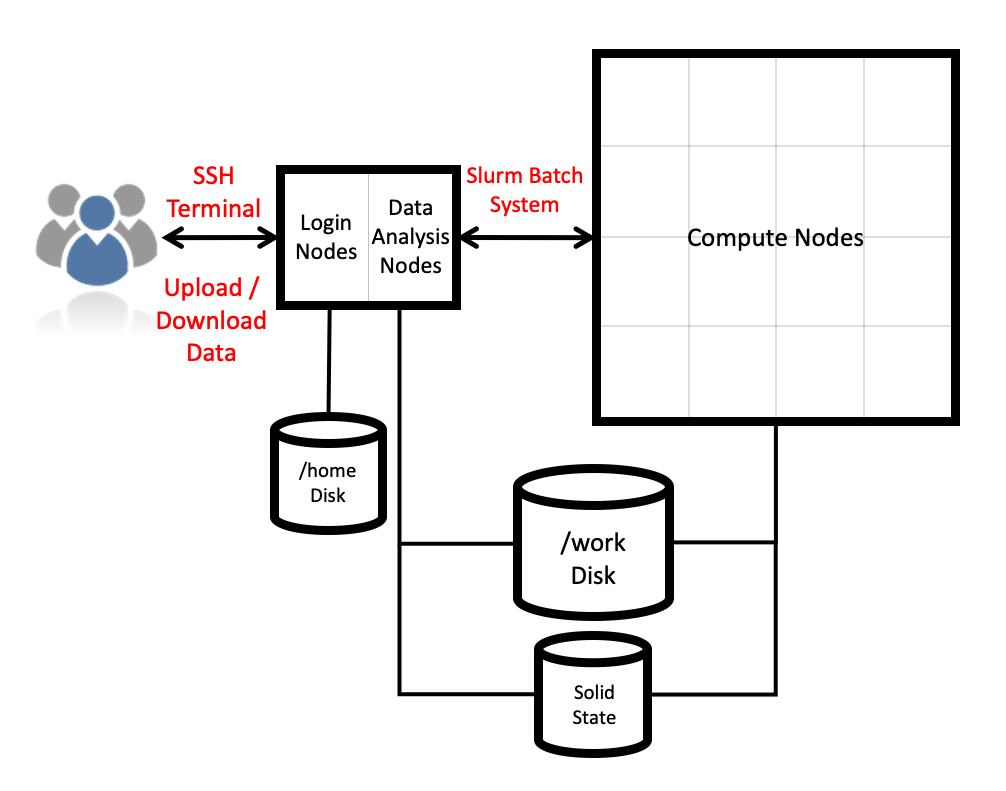
Compute nodes
There are 5,860 CPU compute nodes in total, giving 750,080 compute cores on the full ARCHER2 system. There are also 4 GPU nodes for software development. Most of these (5,276 nodes) have 256 GiB memory per node, a smaller number (584 nodes) have 512 GiB memory per node. All of the compute nodes are linked together using the high-performance HPE Slingshot interconnect.
Access to the compute nodes is controlled by the Slurm scheduling system which supports both batch jobs and interactive jobs.
Compute node summary:
| CPU Nodes | GPU Nodes | |
|---|---|---|
| Processors | 2x AMD EPYC Zen2 (Rome) 7742, 2.25 GHz, 64-core | 1x AMD EPYC Zen3 7543P (Milan), 2.8GHz, 32-core |
| Cores per node | 128 | 32 |
| NUMA | 8 NUMA regions per node, 16 cores per NUMA region | 4 NUMA regions, 8 cores per NUMA region |
| Memory Capacity | 256/512 GiB DDR4 3200MHz, 8 memory channels | 512 GiB DDR4 3200MHz, 8 memory channels |
| Memory Bandwidth | >380 GB/s per node | 40 GB/s (Host-Device), 80GB/s (Device-Device) |
| Interconnect Bandwidth | 25 GB/s per node bi-directional | 25 GB/s per node bi-directional |
| Accelerators | None | 4x AMD Instinct MI210, 104 compute units, 64GiB HBM2e memory |
What is LAMMPS?
LAMMPS (Large-scale Atomic/Molecular Massively Parallel Simulator) is a versatile classical molecular dynamics software package that has been extended to be useful to many other domains, including coarse-grained MD, discrete element method, hydrodynamics, lattice boltzmann, peridynamics, etc. It is developed by Sandia National Laboratories and by its wide user-base under GPLv2.
It can be downloaded from the LAMMPS website
Everything we are covering today (and a lot of other info) can be found in the LAMMPS User Manual
Using a LAMMPS module on ARCHER2
ARCHER2 uses a module system. In general, you can run LAMMPS on
ARCHER2 by using the LAMMPS module. You can use the
module spider command to list all available versions of a
module, and their dependencies:
OUTPUT
---------------------------------------------------------------------
  lammps:
---------------------------------------------------------------------
     Versions:
        lammps/2Aug2024-GPU
        lammps/13Feb2024
        lammps/15Dec2023
        lammps/17Feb2023
        lammps/29Aug2024
     Other possible modules matches:
        cpl-lammps  cpl-openfoam-lammps  lammps-gpu  lammps-python

----------------------------------------------------------------------
  To find other possible module matches execute:

      $ module -r spider '.*lammps.*'

----------------------------------------------------------------------
  For detailed information about a specific "lammps" package
  (including how to load the modules) use the module's full name.
  Note that names that have a trailing (E) are extensions provided
  by other modules.
  For example:

     $ module spider lammps/29Aug2024
----------------------------------------------------------------------
Running module load lammps will set up your environment
to use the default LAMMPS module on ARCHER2. For this course, we will be
using the 29 August, 2024 version of LAMMPS:
Once your environment is set up, you will have access to the
lmp LAMMPS executable. Note that you will only be able to
run this on a single core on the ARCHER2 login node.
Running LAMMPS on ARCHER2 compute nodes
We will now launch a first LAMMPS job from the compute nodes. The login nodes are shared resources on which we have limited the amount of cores that can be used for a job. To run LAMMPS simulations on a large number of cores, we must use the compute nodes.
The /home file system is not accessible from the compute
nodes. As such, we will need to submit our jobs from the
/work directory. Every user has a directory in
/work associated to their project code. For this course,
the project code is ta215, so we all have a directory
called: /work/ta215/ta215/<username> (make sure to
replace username with your username).
We have prepared a number of exercises for today. You can either download these by either:
Exercise 1
For this session, we’ll be looking at
exercises/1-performance-exercise/.
In this directory you will find three files:
-
sub.slurmis a Slurm submission script. This will let you submit jobs to the compute nodes. As written, it will run a single-core job but we will be editing it to run on more cores. -
in.ethanolis the LAMMPS input script that we will be using for this exercise. This script will run a small simulation of 125 ethanol molecules. -
data.ethanolis a LAMMPS data file for a single ethanol molecule. This single molecule will be replicated by LAMMPS to generate the system inside the simulation box.
Why ethanol?
The in.ethanol LAMMPS input that we are using for this
exercise is an easily edited benchmark script used within EPCC to test
system performance. The intention of this script is to be easy to edit
and alter when running on varied core/node counts. By editing the
X_LENGTH, Y_LENGTH, and Z_LENGTH
variables, you can increase the box size substantially. As to the choice
of molecule, we wanted something small and with partial charges –
ethanol seemed to fit both of those.
You can submit your first job on ARCHER2 by running:
You can check the progress of your job by running
squeue --me. Your job state will go from PD
(pending) to R (running) to CG (cancelling).
Once your job is complete, it will have produced a file called
slurm-####.out, which contains the standard output and
standard error produced by your job.
A brief overview of the LAMMPS log file
The job will also produce a LAMMPS log file log.64_cpus.
The name of the file will change when the number of tasks requested in
slurm are changed in the sub.slurm file. In this file, you
will find all of the thermodynamic outputs that were specified in the
LAMMPS thermo_style, as well as some very useful
performance information! We will explore the LAMMPS log file in more
details later but, for now, we will concentrate on the LAMMPS
performance information output at the end of the log file. This will
help us to understand what our simulation is doing, and where we can
speed it up.
Running:
OUTPUT
Performance: 12.825 ns/day, 1.871 hours/ns, 148.442 timesteps/s
100.0% CPU use with 64 MPI tasks x 1 OpenMP threads

MPI task timing breakdown:
Section |  min time  |  avg time  |  max time  |%varavg| %total
---------------------------------------------------------------
Pair    | 0.00020468 | 0.30021    | 2.1814     | 117.6 |  4.44
Bond    | 0.00014519 | 0.044983   | 0.2835     |  39.4 |  0.67
Kspace  | 0.43959    | 2.4307     | 2.7524     |  43.8 | 35.98
Neigh   | 3.608      | 3.6659     | 3.7229     |   1.9 | 54.27
Comm    | 0.091376   | 0.26108    | 0.34751    |  12.6 |  3.87
Output  | 0.0028102  | 0.0029118  | 0.003015   |   0.1 |  0.04
Modify  | 0.011717   | 0.045059   | 0.19911    |  23.7 |  0.67
Other   |            | 0.004113   |            |       |  0.06

Nlocal:        102.516 ave         650 max           0 min
Histogram: 44 12 0 0 0 0 0 1 1 6
Nghost:        922.078 ave        2505 max         171 min
Histogram: 8 24 0 7 17 0 0 0 2 6
Neighs:        18165.4 ave      136714 max           0 min
Histogram: 54 2 0 0 0 0 0 1 2 5

Total # of neighbors = 1162584
Ave neighs/atom = 177.19616
Ave special neighs/atom = 7.3333333
Neighbor list builds = 1000
Dangerous builds not checked
Total wall time: 0:00:13
The ultimate aim is always to get your simulation to run in a sensible amount of time. This often simply means trying to optimise the final value (“Total wall time”), though some people care more about optimising efficiency (wall time multiplied by core count).
Increasing computational resources
The first approach that most people take to increase the speed of their simulations is to increase the computational resources. If your system can accommodate this, doing this can sometimes lead to “easy” improvements. However, this usually comes at an increased cost (if running on a system for which compute is charged) and does not always lead to the desired results.
In your first run, LAMMPS was run on 64 cores. For a large enough
system, increasing the number of cores used should reduce the total run
time. In your sub.slurm file, you can edit the number of
tasks in the line:
to run on a different number of cores. An ARCHER2 node has 128 cores, so you can run LAMMPS on up to 128 cores.
Quick benchmark
As a first exercise, fill in the table below.
| Number of cores | Wall time | Performance (ns/day) |
|---|---|---|
| 1 | ||
| 2 | ||
| 4 | ||
| 8 | ||
| 16 | ||
| 32 | ||
| 64 | ||
| 128 |
Do you spot anything unusual in these run times? If so, can you explain this strange result?
The simulation takes almost the same amount of time when running on a
single core as when running on two cores. A more detailed look into the
in.ethanol file will reveal that this is because the
simulation box is not uniformly packed. We won’t go into all the details
in this course, but we do cover most of the available optimisations in
the advanced course.
Note
Here we are only considering MPI parallelisation. LAMMPS offers the option to run using joint MPI+OpenMP (more on that on the advanced LAMMPS course), but for the exercises in this lesson, we will only be considering MPI.
- “LAMMPS is a versatile software used in a wide range of subjects to run classical molecular dynamics simulations.”
- “Running jobs on ARCHER2 requires a submission to the Slurm batch system using specific account, budget, queue, and qos keywords.”
- “Adding more cores is not always the most effective way of increasing performance.”
Content from Setting up a simulation in LAMMPS
Last updated on 2026-03-31 | Edit this page
Overview
Questions
- “How do we setup a simulation in LAMMPS?”
- “What do all the commands in the input file mean?”
Objectives
- “Understand the commands, keywords, and parameters necessary to setup a LAMMPS simulation.”
Intro to LAMMPS simulations
LAMMPS uses text files as input files that control the setup and flow of a simulation, and a variety of file types (and other methods) initial system for topologies.
Whether the simulation to run is MD or DEM, LAMMPS applies Newton’s laws of motion to systems of particles that can range in size from atoms, course-grained moieties, entire molecules, or even grains of sand. In practical terms, the movement of the particles is calculated by the simple repeating loop:
- Take the initial positions of the particles in the simulation box and calculate the total force that is applied to each particle, using the chosen force-field.
- Use the calculated forces to calculate the acceleration to add to each particle.
- Use the acceleration to calculate the new velocity of each particle.
- Use the the new velocity of each particle, and the defined time-step, to calculate a new position for each particle.
- Repeat ad nauseum.
With the new particle positions, the cycle continues, one very small time-step at a time.
With this in mind, we can take a look at a very simple example of a
LAMMPS input file, in.pour, and discuss each command – and
their related concepts – one by one. The order that the commands appear
in can be important, depending on the exact details.
Always refer to the LAMMPS manual to
check.
For this session, we’ll be looking at the
2-pour-exercise/in.pour file in your exercises
directory.
Simulation setup
The first thing we have to do is chose a style of units. This can be
achieved by the units command:
units ljLAMMPS has several different unit styles, useful in
different types of simulations. In this example, we are using
lj, or Lennard-Jones (LJ) units. These are dimensionless
units, that are defined on the LJ potential parameters. They are
computationally advantageous because they’re usually close to unity, and
required less precise (lower number of bits) floating point variables –
which in turn reduced the memory requirements, and increased calculation
speed.
The next line defines what style of atoms (LAMMPS’s
terminology for particle) to use:
atom_style sphereThe atom style
impacts on what attributes each atom has associated with it – this
cannot be changed during a simulation. Every style stores: coordinates,
velocities, atom IDs, and atom types. The sphere style also
stores radius, mass, omega, and torque for each particle. Other styles
will store additional, or different, information.
We then define the number of dimensions in our system:
dimension 3LAMMPS is also capable of simulating two-dimensional systems.
The boundary command sets the styles for the boundaries for the simulation box.
boundary p p fEach of the three letters after the keyword corresponds to a
direction (x, y, z), and p means that the selected boundary
is to be periodic, while f means it’s fixed, that is,
LAMMPS won’t generate periodic images accross this dimension, and
particles won’t be able to go accross the limits of the simulation box
accross this dimension. Other boundary conditions are available
(shrink-wrapped, and shrink-wrapped with minimum).
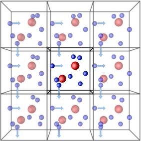
Periodic boundary conditions (PBCs) allow the approximation of an infinite system by simulating only a small part, a unit-cell. The most common shapes of (3D) unit-cell is cuboidal, but any shape that completely tessellates 3D space can be used. The topology of PBCs is such that a particle leaving one side of the unit cell, it reappears on the other side. A 2D map with PBC could be perfectly mapped to a torus.
Another key aspect of using PBCs is the use of the minimum-image convention for calculating interactions between particles. This guarantees that each particle interacts only with the closest image of another particle, no matter with unit-cell (the original simulation box or one of the periodic images) it belongs to.
Granular interactions depend on the velocity of neighbouring particles, so we need to setup LAMMPS to communicate the velocities of “ghost” particles between processors:
comm_modify vel yesThe region command defines a geometric region in space.
region reg block -20 20 -20 20 0 40The arguments are box, a name we give to the region,
block, the type of region (cuboid), and the numbers are the
min and max values for x, y, and z.
We then create a box with two “atom” types, using the region we defined previously
create_box 2 regInter-particle interactions
Now that we have a simulation box, we have to define how particles will interact with each-other once we start adding them to the box.
The first line in this section defines the style of interaction our particles will use.
pair_style granularLAMMPS has a large number of pairwise interparticle interactions available. In this case, we are using the granular pair style, which supports a number of options for normal, tangential, rolling, and twisting forces that result from the contact between particles that need to be setup, using the commands:
pair_coeff      1 * jkr 1000.0 50.0 0.3 10 tangential mindlin 800.0 1.0 0.5 rolling sds 500.0 200.0 0.5 twisting marshall
pair_coeff      2 2 hertz 200.0 20.0 tangential linear_history 300.0 1.0 0.1 rolling sds 200.0 100.0 0.1 twisting marshall
Neighbour lists
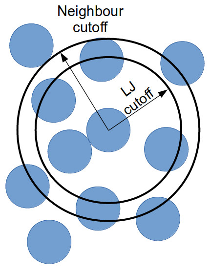
To improve simulation performance, and because we are truncating interactions at a certain distance, we can keep a list of particles that are close to each other (under a neighbour cutoff distance). This reduces the number of comparisons needed per time-step, at the cost of a small amount of memory.
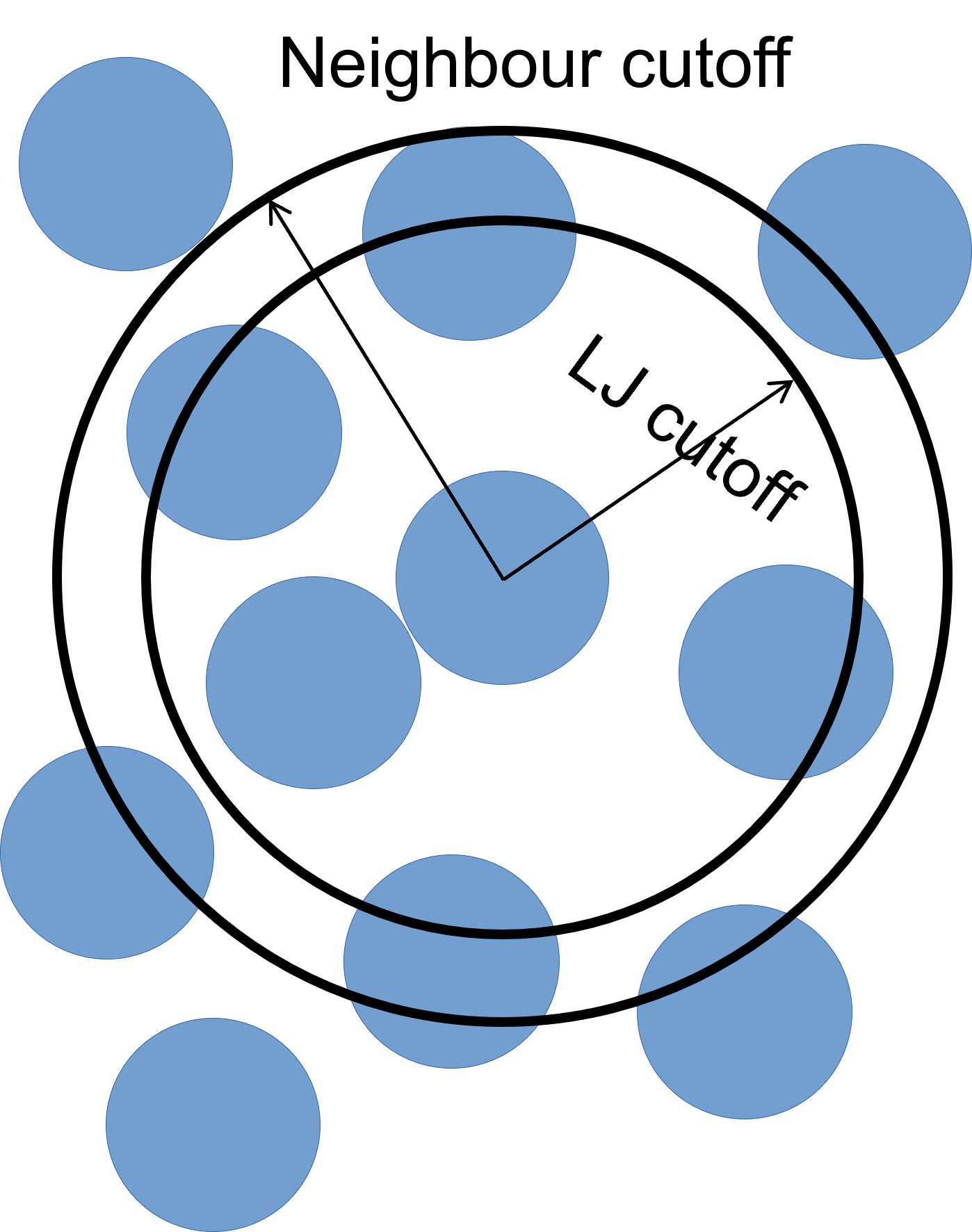
We can set our neighbour list cutoff to be 0.3σ greater than the default cutoff – remember that, as we are dealing with spheres, a small increase in radius results can result in a large volume increase.
The bin keyword refers to the algorithm used to build
the list, bin is the best performing algorithm for systems
with homogeneous sizes of particles, but there are others.
neighbor 0.3 binThese lists still need to be updated periodically. Provided that we
rebuild them more frequently than the minimum time it takes for a
particle to move from within the neighbour cutoff to outside of it. We
use the neigh_modify command to set the wait time between
each neighbour list rebuild:
neigh_modify delay 10 every 1The delay parameter sets the minimum number of
time-steps that need to pass since the last neighbour list rebuild for
LAMMPS to even consider rebuilding it again. The every
parameter tells LAMMPS to attempt to build the neighbour list if the
number of timesteps since the delay ended is equal to the
every value – by default, the rebuild will only be
triggered if an atom has moved more than half the neighbour skin
distance (the 0.3 above).
How to set neighbour list delays?
You can estimate the frequency at which you need to rebuild neighbour lists by running a quick simulation with neighbour list rebuilds every timestep:
and looking at the resultant LAMMPS neighbour list information in the log file generated by that run.
The Neighbour list builds tells you how often neighbour lists needed to be rebuilt. If you know how many timesteps your short simulation ran for, you can estimate the frequency at which you need to calculate neighbour lists by working out how many steps there are per rebuild on average. Provided that your update frequency is less than or equal to that, you should see a speed up.
Simulation parameters
Now that we’ve set up the initial conditions for the simulation, and changed some settings to make sure it runs a bit faster, all that is left is telling LAMMPS exactly how we want the simulation to be run. This includes, but is not limited to, what ensemble to use (and which particles to apply it to), how big the time-step is, how many time-steps we want to simulate, what properties we want as output, and how often we want those properties logged.
The fix command has a myriad of options, most of
them related to ‘setting’ certain properties at a value, or in an
interval of values for one, all, or some particles in the
simulation.
The first keywords are always ID – a name to reference
the fix by, and group-ID – which particles to apply the
command to. The most common option for the second keyword is
all.
fix 1 all nve/sphereThen we have the styles plus the arguments. In the case above, the
style is nve/sphere, and there are no arguments.
Next, we enable gravity on our simulation:
fix grav all gravity 9.8 vector 0 0 -1Pouring particles
To pour particles into our box, we need to setup a region where particles can appear. We can create two cylindrical regions with the commands:
region          cyl1 cylinder z -10  9 10 20 35
region          cyl2 cylinder z  10 -9 10 20 35
Here, the parameters after cylinder are: the direction
of the axis of the cylinder, the coordinates of the axis in the other
two dimensions, the radius, and the low- and high- coordinate along the
axis of the cylinder faces.
Then, we use the fix pour command to create particles in
our simulation box.
#               ID   group-id style n_part type seed kw     region_id kw   d_style min_diam max_diam kw   min_dens max_dens
fix             ins1 all      pour  10000  1    3123 region cyl1      diam range   0.5      1        dens 1.0      1.0
fix             ins2 all      pour  10000  2    4567 region cyl2      diam range   0.5      1        dens 1.0      1.0
Finally, we setup the properties of our bottom wall:
fix 2 all wall/gran granular hertz/material 1e5 1e3 0.3 tangential mindlin NULL 1.0 0.5 zplane 0 NULLFinal setup
To have a valid simulation setup, we need to set the size of the time-step, in whatever units we have chosen for this simulation – in this case, LJ units.
timestep 0.001The size of the time-step is a careful juggling of speed and accuracy. A small time-step guarantees that no particle interactions are missing, at the cost of a lot of computation time. A large time-step allows for simulations that probe effects at longer time scales, but risks a particle moving so much in each time-step, that some interactions are missed – in extreme cases, some particles can ‘fly’ right through each other. The ‘happy medium’ depends on the system type, size, and other variables.
The next line sets what thermodynamic information we want LAMMPS to output to the terminal and the log file.
thermo_style custom step atomsThere are several default styles, and the custom style
allows for full customisation of which fields and in which order to
write them.
In MD simulations (LAMMPS original use-case), losing an atom during
the simulation is a catastrophic mistake, so by default LAMMPS
terminates any simulation that looses particles with an error. To change
this behaviour for DEM simulations, use the thermo_modify
command:
thermo_modify lost ignoreTo set the frequency (in time-steps) at which these results are
output, you can vary the thermo command:
thermo 100In this case, an output will be printed every 100 time-steps.
We can then select how to output the output trajectory files, we give here two distinct options for different visualisation programs:
# for Ovito:
dump            1 all custom 100 dump.pour id type radius mass x y z
# for VTK:
dump            2 all vtk 100 pour*.vtk id type radius mass x y z
dump_modify 2 binary yesNB - Using VTK
For LAMMPS to be able to output in the VTK format, the executable being used needs to have been compiled with the VTK package support. This requires the system being used to have the VTK library installed. The current version of LAMMPS on ARCHER2 does not have VTK support.
And finally, we choose how many time-steps (not time-units) to run the simulation for:
run 10000Run pour simulation
What command does it take to submit the simulation to the ARCHER2 queue? What was the output?
- “LAMMPS can simulate systems of many particles that are allowed to interact, using any of a number of contact models.”
- “A LAMMPS input file is a an ordered collection of commands with both mandatory and optional arguments.”
- “To successfully run a LAMMPS simulation, an input file needs to cover basic simulation setup, read/create a system topology, force-field, and type/frequency of outputs.”
Content from Understanding the logfile
Last updated on 2026-03-31 | Edit this page
Overview
Questions
- “What information does LAMMPS print to screen/logfile?”
- “What does that information mean?”
Objectives
- “Understand the information that LAMMPS prints to screen / writes to the logfile before, during, and after a simulation.”
Log file
The logfile is where we can find thermodynamic information of
interest. By default, LAMMPS will write to a file called
log.lammps. All info output to the terminal is replicated
in this file. We can change the name of the logfile by adding a
log command to your script:
log new_file_name.extensionWe can change which file to write to multiple times during a
simulation, and even append to a file if, for example, we
want the thermodynamic data separate from the logging of other assorted
commands. The thermodynamic data, which we setup with the
thermo and thermo_style command, create the
following (truncated) output:
   Step        Atoms
         0           0
       100        3402
       200        3402
       300        3402
       400        3402
At the start, we get a header with the column names, and then a line
for each time-step that’s a multiple of the value we set
thermo to. In this example we can see the number of
particle change as the simulation progresses. At the end of each
run command, we get the analysis of how the simulation time
is spent:
Loop time of 27.0361 on 128 procs for 10000 steps with 20000 atoms

Performance: 31957.239 tau/day, 369.875 timesteps/s, 7.398 Matom-step/s
99.8% CPU use with 128 MPI tasks x 1 OpenMP threadsLoop time of 27.0361 on 128 procs for 10000 steps with 20000 atoms

MPI task timing breakdown:
Section |  min time  |  avg time  |  max time  |%varavg| %total
---------------------------------------------------------------
Pair    | 0.00044784 | 0.72334    | 18.078     | 340.9 |  2.68
Neigh   | 0.0029201  | 0.059077   | 1.0824     |  73.2 |  0.22
Comm    | 0.94043    | 15.311     | 20.813     | 142.0 | 56.63
Output  | 0.27547    | 0.84274    | 2.1389     |  59.9 |  3.12
Modify  | 5.4303     | 5.6532     | 6.4467     |   7.9 | 20.91
Other   |            | 4.447      |            |       | 16.45

Nlocal:         156.25 ave        2361 max           0 min
Histogram: 110 2 5 7 0 0 0 0 2 2
Nghost:        139.727 ave        1474 max           0 min
Histogram: 108 0 0 8 4 2 2 0 2 2
Neighs:        1340.88 ave       28536 max           0 min
Histogram: 112 7 5 0 0 0 0 0 2 2

Total # of neighbors = 171633
Ave neighs/atom = 8.58165
Neighbor list builds = 1000
Dangerous builds = 994
Total wall time: 0:00:28
The data shown here is very important to understand the computational
performance of our simulation, and we can it to help improve the speed
at which our simulations run substantially. The first line gives us the
details of the last run command - how many seconds it took,
on how many processes it ran on, how many time-steps, and how many
atoms. This can be useful to compare between different systems.
Then we get some benchmark information:
Performance: 31957.239 tau/day, 369.875 timesteps/s, 7.398 Matom-step/s
99.8% CPU use with 128 MPI tasks x 1 OpenMP threadsLoop time of 27.0361 on 128 procs for 10000 steps with 20000 atoms
This tells us how many time units per day, how many time-steps per second we are running, and how many “Mega-atom-step per second” which is an easier measure to compare systems of different sizes (i.e., number of particles). It also tells us how much of the available CPU resources LAMMPS was able to use, and how many MPI tasks and OpenMP threads.
The next table shows a breakdown of the time spent on each task by the MPI library:
MPI task timing breakdown:
Section |  min time  |  avg time  |  max time  |%varavg| %total
---------------------------------------------------------------
Pair    | 0.00044784 | 0.72334    | 18.078     | 340.9 |  2.68
Neigh   | 0.0029201  | 0.059077   | 1.0824     |  73.2 |  0.22
Comm    | 0.94043    | 15.311     | 20.813     | 142.0 | 56.63
Output  | 0.27547    | 0.84274    | 2.1389     |  59.9 |  3.12
Modify  | 5.4303     | 5.6532     | 6.4467     |   7.9 | 20.91
Other   |            | 4.447      |            |       | 16.45
There are 8 possible MPI tasks in this breakdown:
-
Pairrefers to non-bonded force computations -
Bondincludes all bonded interactions, (so angles, dihedrals, and impropers) -
Kspacerelates to long-range interactions (Ewald, PPPM or MSM) -
Neighis the construction of neighbour lists -
Commis inter-processor communication (AKA, parallelisation overhead) -
Outputis the writing of files (log and dump files) -
Modifyis the fixes and computes invoked by fixes -
Otheris everything else
Each category shows a breakdown of the least, average, and most
amount of wall time any processor spent on each category – large
variability in this (calculated as %varavg) indicates a
load imbalance (which can be caused by the atom distribution between
processors not being optimal). The final column, %total, is
the percentage of the loop time spent in the category.
A rule-of-thumb for %total on each category
-
Pairandmodify: as much as possible. -
NeighandComm: as little as possible. If it’s growing large, it’s a clear sign that too many computational resources are being assigned to a simulation.
The next section is about the distribution of work amongs the different threads:
Nlocal:         156.25 ave        2361 max           0 min
Histogram: 110 2 5 7 0 0 0 0 2 2
Nghost:        139.727 ave        1474 max           0 min
Histogram: 108 0 0 8 4 2 2 0 2 2
Neighs:        1340.88 ave       28536 max           0 min
Histogram: 112 7 5 0 0 0 0 0 2 2
The three subsections all have the same format: a title followed by
average, maximum, and minimum number of particles per processor,
followed by a 10-bin histogram of showing the distribution. The total
number of histogram counts is equal to the number of processors used.
The three properties listed are: - Nlocal: number of owned
atoms; - Nghost: number of ghost atoms; -
Neighs: pairwise neighbours.
The final section shows aggregate statistics accross all processors for pairwise neighbours:
Total # of neighbors = 171633
Ave neighs/atom = 8.58165
Neighbor list builds = 1000
Dangerous builds = 994
It includes the number of total neighbours, the average number of
neighbours per atom, the number of neighbour list rebuilds, and the
number of potentially dangerous rebuilds. The potentially
dangerous rebuilds are ones that are triggered on the first
timestep that is checked. If this number is not zero, you should
consider reducing the delay factor on the neigh_modify
command.
The last line on every LAMMPS simulation will be the total wall time
for the entire input script, no matter how many run
commands it has:
Total wall time: 0:00:28- “Thermodynamic information outputted by LAMMPS can be used to track whether a simulations is running OK.”
- “Performance data at the end of a logfile can give us insights into how to make a simulation faster.”
Content from Advanced input and output commands
Last updated on 2026-03-31 | Edit this page
Overview
Questions
- “How do I calculate a property every N time-steps?”
- “How do I write a calculated property to file?”
- “How can I use variables to make my input files easier to change?”
Objectives
- “Understand the use of
compute,fix, and variables.”
Advanced input commands
LAMMPS has a very powerful suite for calculating, and outputting all
kinds of physical properties during the simulation. Calculations are
most often under a compute command, and
then the output is handled by a fix command. We will now
look at some examples, but there are (at the time of writing) over 150
different compute commands with many options each.
LAMMPS trajectory files
We can output information about a group of particles in our system by
using the LAMMPS dump command. In this example, we will be
outputting the particle positions, but you can output many other
attributes, such as particle velocities, types, angular momentum, etc.
The list of attributes (and examples of dump commands) can
be found in the relevant
LAMMPS manual page.
If we look at the starting input script in
exercises/3-advanced-inputs-exercise/in.lj_start, we find
that the following command has been added:
dump 1 all custom 100 rotating_drum.dump id type radius mass x y zThe dump command defines the properties that we want to
output, and how frequently we want these output. In this case, we have
set the ID of the dump command to 1 (we could
have used any name/number and it would still work). We want to output
properties for all particles in our system. We’ve set the
output type to custom to have better control of what’s
being output – there are default dump options but
custom is generally the one that gets used. We’ll be
outputting every 100 time-steps to a file called
nvt.lammpstrj – a *.lammpstrj file can be
recognised by some post-processing and post-analysis tools as a LAMMPS
trajectory/dump file, and can save some time down the line. Finally, we
name the properties we want to output – in this case, we want to output
the particle ID, type, (x,y,z) components of position, and the (x, y, z)
components of velocity.
We’ve added a dump_modify command to get LAMMPS to sort
the output by ID order – we tell the dump_modify command
which dump command we’d like to sort by giving the dump-ID
(in this case, our dump command had an ID of
1). We then specify how we want to modify this
dump command – we want to sort it by ID, but
there are many more options (that you can find in the LAMMPS manual).
The output rotating_drum.dump file looks like this:
ITEM: TIMESTEP
100
ITEM: NUMBER OF ATOMS
2741
ITEM: BOX BOUNDS pp pp ff
0.0000000000000000e+00 3.0000000000000000e+01
0.0000000000000000e+00 3.0000000000000000e+01
0.0000000000000000e+00 3.0000000000000000e+01
ITEM: ATOMS id type radius mass x y z
1 1 0.388095 0.244852 25.2758 16.9939 28.3519
2 1 0.485033 0.477973 24.1818 24.6876 27.6903
3 1 0.423595 0.318376 13.2428 21.4007 19.1017
4 1 0.353413 0.184899 7.58115 10.3236 26.5067
5 1 0.434095 0.342644 10.5736 17.2751 19.3327
The lines with ITEM: let you know what is output on the
next lines (so ITEM: TIMESTEP lets you know that the next
line will tell you the time-step for this frame – in this case,
100,000). A LAMMPS trajectory file will usually contain the time-step,
number of atoms, and information on box bounds before outputting the
information we’d requested.
Restart files
To allow the continuation of the simulation (with the caveat that it must continue to run in the same number of cores as was originally used), we can create a restart file.
This binary file contains information about system topology, force-fields, but not about computes, fixes, etc, these need to be re-defined in a new input file.
You can write a restart file with the command:
write_restart drum.restartAn arguably better solution is to write a data file, which not only is a text file, but can then be used without restrictions in a different hardware configuration, or even LAMMPS version.
write_data drum.dataYou can use a restart or data file to start/restart a simulation by
using a read command. For example:
read_restart drum.restartwill read in our restart file and use that final point as the starting point of our new simulation.
Similarly:
read_data drum.datawill do the same with the data file we’ve output (or any other data file).
Radial distribution functions (RDFs)
Next, we will look at the Radial Distribution Function (RDF), g(r). This describes how the density of a particles varies as a function of the distance to a reference particle, compared with a uniform distribution (that is, at r → ∞, g(r) → 1). We can make LAMMPS compute the RDF by adding the following lines to our input script:
compute        RDF all rdf 150 cutoff 3.5
fix            RDF_OUTPUT all ave/time 25 100 5000 c_RDF[*] file rdf.out mode vector
We’ve named this compute command RDF and
are applying it to the atom-group all. The compute is of
style rdf, and we have set it to have with 150 bins for the
RDF histogram (e.g. there are 150 discrete distances at which atoms can
be placed). We’ve set a maximum cutoff of 3.5σ, above which we stop
considering particles.
Compute commands are instantaneous – they calculate the values for
the current time-step, but that doesn’t mean they calculate quantities
every time-step. A compute only calculates quantities when needed,
i.e., when called by another command. In this case, we will use
our compute with the fix ave/time command, that averages a
quantity over time, and outputs it over a long timescale.
Our fix ave/time has the following parameters: -
RDF_OUTPUT is the name of the fix, all is the
group of particles it applies to. - ave/time is the style
of fix (there are many others). - The group of three numbers
25 100 5000 are the Nevery,
Nrepeat, Nfreq arguments. These can be quite
tricky to understand, as they interplay with each other. -
Nfreq is how often a value is written to file. -
Nrepeat is how many sets of values we want to average over
(number of samples) - Nevery is how many time-steps in
between samples. - Nfreq must be a multiple of
Nevery, and Nevery must be non-zero even if
Nrepeat = 1. - So, for example, an Nevery of
2, with Nrepeat of 3, and Nfreq of 100: at
every time-step multiple of 100 (Nfreq), there will be an
average written to file, that was calculated by taking 3 samples
(Nrepeat), 2 time-steps apart (Nevery). So,
time-steps 96, 98, and 100 are averaged, and the average is written to
file. Likewise at time-steps 196, 198, and 200, etc. - In this case, we
take a sample every 25 time-steps, 100 times, and output at time-step
number 5000 – so from time-step 2500 to 5000, sampling every 25
time-steps. - c_RDF[*], is the compute that we want to
average over time. c_ defines that we’re wanting to use a
compute, and RDF is our compute name. The [*]
wildcard in conjunction with mode vector makes the fix
calculate the average for all the columns in the compute ID. - The
file rdf_lj.out argument tells LAMMPS where to write the
data to.
For this command, the file looks something like this:
OUTPUT
# Time-averaged data for fix RDF_OUTPUT
# TimeStep Number-of-rows
# Row c_RDF[1] c_RDF[2] c_RDF[3]
100000 150
1 0.0116667 0 0
2 0.035 0 0
3 0.0583333 0 0
4 0.0816667 0 0
5 0.105 0 0
...
20 0.455 0 0
21 0.478333 0.334462 0.00227339
22 0.501667 1.9594 0.0169225
23 0.525 3.49076 0.0455044
24 0.548333 7.58762 0.113275
25 0.571667 9.36566 0.204196
...YAML output
Since version 4May2022 of LAMMPS, writing to YAML files support was
added. To write a YAML file, just change the extension accordingly
file rdf_lj.yaml. The file will then be in YAML format:
Variables and loops
LAMMPS input scripts can be quite complex, and it can be useful to run the same script many times with only a small difference (for example, temperature). For this reason, LAMMPS have implemented variables and loops – but this doesn’t mean that we can only use variables with loops.
A variable in LAMMPS is defined with the keyword
variable, then a name, and then style and
arguments, for example:
variable        StepsPerRotation equal 20000.0
variable        theta equal 2*PI*elapsed/${StepsPerRotation}
There are several variable styles. Of
particular note are: - equal is the workhorse of the
styles, and it can set a variable to a number, thermo
keywords, maths operators or functions, among other things. -
delete unsets a variable. - loop and
index are similar, and will result in the variable changing
to the next value in a list every time a next command is
seen. The difference that loop accepts an integer or range,
while index accepts a list of strings.
To use a variable later in the script, just prepend a dollar sign, like so:
thermo_style custom step atoms ke v_thetaExample of loop:
variable a loop 10
label loop
dump 1 all atom 100 file.$a
run 10000
undump 1
next a
jump SELF loop
and of index:
variable d index run1 run2 run3 run4 run5 run6 run7 run8
label loop
shell cd $d
read_data data.polymer
run 10000
shell cd ..
clear
next d
jump SELFRun drum at several speeds
Modify the files from exercise 3 to use a loop like described above that rotates the drum at different speeds, for example, 5000, 10000, and 20000 steps per rotation.
OUTPUT
# loop
variable        StepsPerRotation index 5000.0 10000.0 20000.0
label loop
# rotate drum
variable        theta equal 2*PI*elapsed/${StepsPerRotation}

dump            2 all custom 100 rotating_drum.$(2*PI/v_StepsPerRotation:%.5f).dump id type radius mass x y z

# run rotation
run             40000

undump 2
next StepsPerRotation
jump SELF loop- “Using
computeandfixcommands, it’s possible to calculate myriad properties during a simulation.” - “Variables make it easier to script several simulations.”
Content from Measuring and improving LAMMPS performance
Last updated on 2026-03-31 | Edit this page
Overview
Questions
- “How can we improve the performance of LAMMPS?”
Objectives
- “Gain an overview of submitting and running jobs on the ARCHER2 service.”
- “Gain an overview of methods to improve the performance of LAMMPS.”
Performance inprovements
There are many configurable parameters in LAMMPS that can lead to changes in performance. Some depend on the system being simulated, others on the hardware being used. Here we will try to cover the most relevant, using the ethanol system from the first exercise.
Domain decomposition
In the earlier exercise, you will (hopefully) have noticed that, while the simulation run time decreases overall as the core count is increased, the run time was the same when run on one processor as it was when run on two processors. This unexpected behaviour (for a truly strong-scaling system, you would expect the simulation to run twice as fast on two cores as it does on a single core) can be explained by looking at our starting simulation configuration and understanding how LAMMPS handles domain decomposition.
In parallel computing, domain decomposition describes the methods used to split calculations across the cores being used by the simulation. How domain decomposition is handled varies from problem to problem. In the field of molecular dynamics (and, by extension, within LAMMPS), this decomposition is done through spatial decomposition – the simulation box is split up into a number of blocks, with each block being assigned to their own core.
By default, LAMMPS will split the simulation box into a number of equally sized blocks and assign one core per block. The amount of work that a given core needs to do is directly linked to the number of atoms within its part of the domain. If a system is of uniform density (i.e., if each block contains roughly the same number of particles), then each core will do roughly the same amount of work and will take roughly the same amount of time to calculate interactions and move their part of the system forward to the next timestep. If, however, your system is not evenly distributed, then you run the risk of having a number of cores doing all of the work while the rest sit idle.
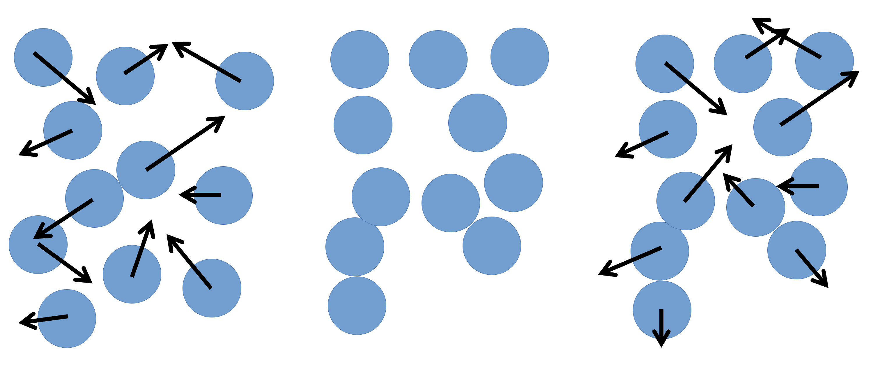
The system we have been simulating looks like this at the start of the simulation:
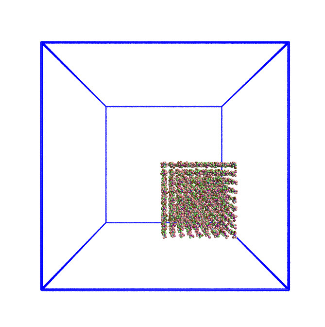
As this is a system of non-uniform density, the default domain decomposition will not produce the desired results.
LAMMPS offers a number of methods to distribute the tasks more evenly
across the processors. If you expect the distribution of atoms within
your simulation to remain constant throughout the simulation, you can
use a balance command to run a one-off re-balancing of the
simulation across the cores at the start of your simulation. On the
other hand, if you expect the number of atoms per region of your system
to fluctuate (e.g. as is common in evaporation), you may wish to
consider recalculating the domain decomposition every few timesteps with
the dynamic fix balance command.
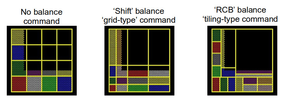
For both the static, one-off balance and the dynamic
fix balance commands, LAMMPS offers two methods of load
balancing – the “grid-like” shift method and the “tiled”
rcb method. The diagram below helps to illustrate how these
work.
Using better domain decomposition
In your in.ethanol file, uncomment the
fix balance command and rerun your simulations. What do you
notice about the runtimes? We are using the dynamic load balancing
command – would the static, one-off balance command be
effective here?
The runtimes decrease significantly when running with dynamic load balancing. In this case, static load balancing would not work as the ethanol is still expanding to fill the simulation box. Once the ethanol is evenly distributed within the box, you can remove the dynamic load balancing.
Playing around with dynamic load balancing
In the example, the fix balance is set to be
recalculated every 1,000 timesteps. How does the runtime vary as you
change this value? I would recommend trying 10, 100, and 10,000.
The simulation time can vary drastically depending on how often re-balancing is carried out. When using dynamic re-balancing, there is an important trade-off between the time gained from re-balancing and the cost involved with recalculating the load balance among cores.
You can find more information about how LAMMPS handles domain decomposition in the LAMMPS manual balance, and fix balance sections.
Considering neighbour lists
Let’s take another look at the profiling information provided by LAMMPS:
Section |  min time  |  avg time  |  max time  |%varavg| %total
---------------------------------------------------------------
Pair    | 68.063     | 68.063     | 68.063     |   0.0 | 34.51
Bond    | 5.0557     | 5.0557     | 5.0557     |   0.0 |  2.56
Kspace  | 5.469      | 5.469      | 5.469      |   0.0 |  2.77
Neigh   | 115.22     | 115.22     | 115.22     |   0.0 | 58.43
Comm    | 1.4039     | 1.4039     | 1.4039     |   0.0 |  0.71
Output  | 0.00034833 | 0.00034833 | 0.00034833 |   0.0 |  0.00
Modify  | 1.8581     | 1.8581     | 1.8581     |   0.0 |  0.94
Other   |            | 0.139      |            |       |  0.07
There are 8 possible MPI tasks in this breakdown:
-
Pairrefers to non-bonded force computations. -
Bondincludes all bonded interactions, (so angles, dihedrals, and impropers). -
Kspacerelates to long-range interactions (Ewald, PPPM or MSM). -
Neighis the construction of neighbour lists. -
Commis inter-processor communication (AKA, parallelisation overhead). -
Outputis the writing of files (log and dump files). -
Modifyis the fixes and computes invoked by fixes. -
Otheris everything else.
Each category shows a breakdown of the least, average, and most
amount of wall time any processor spent on each category – large
variability in this (calculated as %varavg) indicates a
load imbalance (which can be caused by the atom distribution between
processors not being optimal). The final column, %total, is
the percentage of the loop time spent in the category.
In the example above, we notice that the majority of the time is
spent in the Neigh section – e.g. a lot of time is spent
calculating neighbour lists. Neighbour lists are a common method for
speeding up simulations with short-ranged particle-particle
interactions. Most interactions are based on inter-particle distance and
traditionally the distance between every particle and every other
particle would need to be calculated every timestep (this is an \(O(N^2)\) calculation!). Neighbour lists are
a way to reduce this to an \(\sim
O(N)\) calculation for truncated short-ranged interactions.
Instead of considering all interactions between every particle in a
system, you can generate a list of all particles within the truncation
cutoff plus a little bit more. Depending on the size of that “little bit
more” and the details of your system, you can work out how quickly a
particle that is not in this list can move to be within the short-ranged
interaction cutoff. With this time, you can work out how frequently you
need to update this list.
Doing this reduces the number of times that all inter-particle distances need to be calculated: every few timestep, the inter-particle distances for all particle pairs are calculated to generate the neighbour list for each particle; and in the interim, only the inter-particle distances for particles within a neighbour list need be calculated (as this is a much smaller proportion of the full system, this greatly reduces the total number of calculations).
If we dig a bit deeper into our in.ethanol LAMMPS input
file, we will notice the following lines:
variable        NEIGH_TIME  equal      1    # neigh_modify every x dt

...

neigh_modify    delay 0 every ${NEIGH_TIME} check no
These lines together indicate that LAMMPS is being instructed to rebuild the full neighbour list every timestep (so this is not a very good use of neighbour lists).
Changing neighbour list update frequency
Change the NEIGH_TIME variable to equal 10. How does
this affect the simulation runtime?
Now change the NEIGH_TIME variable to equal 1000. What
happens now?
Neighbour lists only give physical solutions when the update time is less than the time it would take for a particle outwith the neighbour cutoff to get to within the short-ranged interaction cutoff. If this happens, the results generated by the simulation become questionable at best and, in the worst case, LAMMPS will crash.
You can estimate the frequency at which you need to rebuild neighbour lists by running a quick simulation with neighbour list rebuilds every timestep:
neigh_modify delay 0 every 1 check yesand looking at the resultant LAMMPS neighbour list information in the log file generated by that run.
Total # of neighbors = 1313528
Ave neighs/atom = 200.20241
Ave special neighs/atom = 7.3333333
Neighbor list builds = 533
Dangerous builds = 0
The Neighbor list builds tells you how often neighbour
lists needed to be rebuilt. If you know how many timesteps your short
simulation ran for, you can estimate the frequency at which you need to
calculate neighbour lists by working out how many steps there are per
rebuild on average. Provided that your update frequency is less than or
equal to that, you should see a speed up.
In this section, we only considered changing the frequency of
updating neighbour lists. Two other factors that can contribute to the
time taken to calculate neighbour lists are the pair_style
cutoff distances (where applicable) and the neighbor skin
distance. Decreasing either of these will reduce the number of particles
within the neighbour cutoff distance, thereby decreasing the number of
interactions being calculated each timestep. However, decreasing these
will mean that lists need to be rebuilt more frequently – it’s always a
fine balance.
You can find more information in the LAMMPS manual about neighbour lists and the neigh_modify command.
Submitting multiple sruns in one job
Jobs on ARCHER2 are charged by the node-hour. However, some
simulation systems are not big enough to justify a full node’s worth of
cores (128). In these cases, we can launch several srun
calls in one batch job, allowing us to make better use of the
computational resources.
Here is what the submission script for the in.ethanol
benchmarking that we used in an earlier lesson looks like, when we
launch all the powers of two number of cores, between 1 and 64, in one
single node:
BASH
#!/bin/sh
#SBATCH --job-name=lmp_ex5
#SBATCH --nodes=1
#SBATCH --time=0:10:0
#SBATCH --hint=nomultithread
#SBATCH --distribution=block:block

# The budget code of the project
#SBATCH --account=ta215
# Standard partition
#SBATCH --partition=standard
# Short QoS since our runtime is under 20m
#SBATCH --qos=short

# load the lammps module
module load lammps/29Aug2024

# Set the number of threads to 1
#   This prevents any threaded system libraries from automatically
#   using threading.
export OMP_NUM_THREADS=1

# setup loop
for i in $(seq 0 6)
do
  cores=$((2**$i))
  echo "Running seq ${i}: ${cores} cpu cores"
  srun --nodes=1 --ntasks=${cores} --ntasks-per-node=${cores} --cpus-per-task=1 --exact \
          --mem=12500M lmp -i in.ethanol -l log.${cores}_cpus &
done

# wait for all jobs to finish
wait
Hybrid MPI+OpenMP runs
When looking at the LAMMPS profiling information, we briefly
mentioned that the proportion of time spent calculating
Kspace should fall within the 10-30% region.
Kspace can often come to dominate the time profile when
running with a large number of MPI ranks. This is a result of the way
that LAMMPS handles the decomposition of k-space across multiple MPI
ranks.
One way to overcome this problem is to run your simulation using
hybrid MPI+OpenMP. To do this, you must ensure that you have compiled
LAMMPS with the OMP package. On ARCHER2, you can edit the
run.slurm file that you have been using to include the
following:
BASH
#SBATCH --tasks-per-node=64
#SBATCH --cpus-per-task=2

...

export OMP_NUM_THREADS=2
export SRUN_CPUS_PER_TASK=$SLURM_CPUS_PER_TASK

srun lmp -sf omp -i in.ethanol -l ${OMP_NUM_THREADS}_log.out
Setting the variable OMP_NUM_THREADS will let LAMMPS
know how many OpenMP threads will be used in the simulation. Setting
--tasks-per-node and --cpus-per-task will
ensure that Slurm assigns the correct number of MPI ranks and OpenMP
threads to the executable. Setting the LAMMPS --sf omp flag
will result in LAMMPS using the OMP version of any command
in your LAMMPS input script.
Running hybrid jobs efficiently can add a layer of complications, and a number of additional considerations must be taken into account to ensure the desired results. Some of these are:
- The product of the values assigned to
--tasks-per-nodeand--cpus-per-taskshould be less than or equal to the number of cores on a node (on ARCHER2, that number is 128 cores). - You should try to restrict the number of OpenMP threads per MPI task to fit on a single socket. For ARCHER2, the sockets (processors) are so large that they have been subdivided into a number of NUMA regions. Each ARCHER2 node 2 sockets, each socket has 4 NUMA regions, each of which has 16 cores, for a total of 8 NUMA regions per node. Therefore, for an efficient LAMMPS run, you would not want to use more than 16 OpenMP processes per MPI task.
- In a similar vein to the above, you also want to make sure that your OpenMP threads are kept within a single NUMA region. Spanning across multiple NUMA regions will decrease the performance (significantly).
These are only some of the things to bear in mind when considering using hybrid MPI+OpenMP to speed up calculations.
- “LAMMPS offers a number of built in methods to improve performance.”
- “It is important to spend some time understanding your system and considering its performance.”
- “Where possible, always run a quick benchmark of your system before setting up a large run.”
Content from Compiling LAMMPS
Last updated on 2026-03-31 | Edit this page
Overview
Questions
- “How can I compile LAMMPS using CMake”
- “How do I build LAMMPS with its shared libraries?”
Objectives
- “Know how to compile LAMMPS on ARCHER2 (and what to look for when compiling elsewhere).”
Building LAMMPS with Python
For this course, we will be using a version of LAMMPS that has been built with the “Python” package and with shared libraries. These will help us ensure that we can run LAMMPS through Python.
The build instructions used can be found in the hpc-uk github and were:
BASH
# select centrally installed modules needed for compilation
module load cpe/22.12
module load cray-fftw/3.3.10.3
module load cmake/3.21.3
module load cray-python

# Add cray library paths to the LD_LIBRARY_PATH variable
export LD_LIBRARY_PATH=$CRAY_LD_LIBRARY_PATH:$LD_LIBRARY_PATH

# clone the chosen version of LAMMPS
git clone --depth=1 --branch stable_15Dec2023 https://github.com/lammps/lammps.git lammps-src-2023-12-15

# create and source a virtual environment
python -m venv --system-site-packages  /work/y07/shared/apps/core/lammps/15_Dec_2023/venv/lammps-python-15-Dec-2023
source /work/y07/shared/apps/core/lammps/15_Dec_2023/venv/lammps-python-15-Dec-2023/bin/activate

# creata folder for configuration and compilation
cd lammps-2023-12-15 && mkdir build_cpe && cd build_cpe

# use cmake to configure LAMMPS
cmake -C ../cmake/presets/most.cmake                                       \
      -D BUILD_MPI=on                                                      \
      -D BUILD_SHARED_LIBS=yes                                             \
      -D CMAKE_CXX_COMPILER=CC                                             \
      -D CMAKE_CXX_FLAGS="-O2"                                             \
      -D CMAKE_INSTALL_PREFIX=/path/to/install  \
      -D FFT=FFTW3                                                         \
      -D FFTW3_INCLUDE_DIR=${FFTW_INC}                                     \
      -D FFTW3_LIBRARY=${FFTW_DIR}/libfftw3_mpi.so                         \
      -D PKG_MPIIO=yes                                                     \
      ../cmake/

make -j 8
make install
make install-python
Of note here:
-
-D CMAKE_INSTALL_PREFIX=/path/to/installdefines the path into which your LAMMPS executables and libraries will be built. You will need to change/path/to/installto whatever you like. -
-D BUILD_SHARED_LIBS=yeswill build the shared LAMMPS library required to run LAMMPS in Python. -
-D PKG_PYTHON=yeswill build the Python packages. - The
-C ../cmake/presets/most.cmakecommand adds the packages that we are installing. Not all of them are required for this course, but it includes all packages that don’t need extra libraries. - The rest of the instructions are to ensure that the correct compiler is used, the MPI version of LAMMPS is built, and that it has access to the correct fast Fourier transform (FFTW) and Eigen3 libraries.
Once this is built, you should be able to run LAMMPS from the compute nodes by loading the appropriate module.
Building LAMMPS with VTK - local linux system
To vuild LAMMPS with VTK on an Ubuntu/Debian system (or virtual machine), you will need to install the following pre-requesites:
- Compiler (gcc or clang)
- MPI
- VTK
- FFTW3
- Optionally, python
To do this, you can use the aptitude package manager:
Regular MPI executable and python wrappers
Create and go into a build directory:
Build using:
Building LAMMPS with VTK on ARCHER2
These instructions are for building LAMMPS version 13Feb2024, also known as 07Feb2024 update 1, on ARCHER2 using the Cray clang compilers 15.0.2 // cpe 22.12 with support for VTK files.
Path setup
BASH
# base-path for download and source files
export DWNLD_DIR="/work/ta215/ta215/shared/download"
export INSTALL_DIR="/work/ta215/ta215/shared/"
export LAMMPS_DWNLD=${DWNLD_DIR}/lammps-2024-02-13
export LAMMPS_BUILD=${LAMMPS_DWNLD}/build
export LAMMPS_INSTALL=${INSTALL_DIR}/lammps
export VTK_DWNLD=${DWNLD_DIR}/vtk
export VTK_BUILD=${VTK_DWNLD}/build
export VTK_INSTALL=${INSTALL_DIR}/vtk-9.5.2
Setup your environment
Load the correct modules:
BASH
module load cpe/22.12
module load cray-fftw/3.3.10.3
module load cmake/3.21.3
module load cray-python

export LD_LIBRARY_PATH=$CRAY_LD_LIBRARY_PATH:$LD_LIBRARY_PATH

# create and source a virtual environment
python -m venv --system-site-packages ${LAMMPS_INSTALL}/venv/lammps-python-13-Feb-2024
source ${LAMMPS_INSTALL}/venv/lammps-python-13-Feb-2024/bin/activate
Download and compile the VTK library
BASH
mkdir -p ${VTK_DWNLD}
cd ${VTK_DWNLD}
wget https://vtk.org/files/release/9.5/VTK-9.5.2.tar.gz
tar -xvf VTK-9.5.2.tar.gz
mv VTK-9.5.2 source
mkdir -p ${VTK_BUILD}
cd ${VTK_BUILD}
cmake -DVTK_USE_MPI:BOOL=ON -DVTK_SMP_IMPLEMENTATION_TYPE:STRING=OpenMP -DCMAKE_BUILD_TYPE:STRING=Release ${VTK_DWNLD}/source
cmake --build . -j8
cp -r ${VTK_DWNLD} ${VTK_INSTALL}Regular MPI executable and python wrappers
Create and go into a build directory:
Build using:
BASH
cmake -C ../cmake/presets/most.cmake                \
      -D BUILD_MPI=on                               \
      -D BUILD_SHARED_LIBS=yes                      \
      -D CMAKE_CXX_COMPILER=CC                      \
      -D CMAKE_CXX_FLAGS="-O2"                      \
      -D CMAKE_INSTALL_PREFIX=${LAMMPS_INSTALL}     \
      -D FFT=FFTW3                                  \
      -D FFTW3_INCLUDE_DIR=${FFTW_INC}              \
      -D FFTW3_LIBRARY=${FFTW_DIR}/libfftw3_mpi.so  \
      -D PKG_MPIIO=yes                              \
      -D PKG_VTK=yes                                \
      -D VTK_DIR=${VTK_INSTALL}                     \
      ../cmake/

make -j 8
make install
make install-pythonTo run LAMMPS from python
LD_PRELOAD needs to be modified (this is done in the
module file, but if running the text below without loading a module, it
needs to be done explicitly):
- “Compiling LAMMPS with CMake is easy and quick on ARCHER2”
Content from Running LAMMPS through Python
Last updated on 2026-03-31 | Edit this page
Overview
Questions
- “How can I run LAMMPS from within Python?”
Objectives
- “Know how run a LAMMPS simulation through Python.”
Running LAMMPS through Python
Running LAMMPS through Python is quite a simple task: you can import the LAMMPS Python library, start the LAMMPS environment, and run a LAMMPS simulation by running the following commands:
PYTHON
from lammps import lammps

def main():
    lmp = lammps()
    lmp.file("in.pour")

if __name__ == '__main__':
    main()
Python will use the shared LAMMPS libraries to run this. Under the hood, LAMMPS runs the same processes as it would if the script was run directly through the LAMMPS executable, and jobs run with Python will run in comparable times.
One of the main advantages of running LAMMPS through Python is that
it allows you to make use of Python’s dynamic programming. Also, while
LAMMPS offers a large amount of options for writing scripts (via
e.g. variables definition, jump commands and
if statements), these are not as intuitive to a lot of
users as a Python interface.
Exercise
We have prepared an example on how to call LAMMPS from python. To
access this, please cd exercises/6-python/. In this
directory you will find three files:
-
in.drumis the LAMMPS input file adapted from an earlier exercise with a rotating drum. -
lammps_drum.pyis a Python script that initially runs the simulation defined in thein.drumLAMMPS configuration file. Once that is complete, the script will launch a series of simulations run with changing rotating drum speeds -
sub.slurmis the Slurm submission script for running this simulation on the ARCHER2 compute nodes.
You can submit this simulation to the queue by running:
One disadvantage of using the LAMMPS python module is that debugging can be more complicated when things go wrong. There are more moving parts than with the LAMMPS executable, and it can often be difficult to trace back errors and attribute them correctly to LAMMPS, Python, or the interface.
The LAMMPS python module has a number of other features and variables that can be called to improve your use of LAMMPS through Python. You can find more information about this in the LAMMPS manual.
- “Running LAMMPS through Python can have certain advantages.”
- “However, finding the root cause of problems when things go wrong is harder to do when running LAMMPS through Python rather than through a LAMMPS executable.”