Credits

Exercise content created by EPCC, The University of Edinburgh. Documentation and source code copyright The University of Edinburgh 2019. Lab style and template created by NVIDIA, see https://nvidia.qwiklab.com/.

Purpose

In this self-paced, hands-on lab, we will take an existing CUDA application and go through several optimization steps, measuring the performance benefits of each. We will see the importance of minimizing data transfer, enabling coalesced memory access, and tuning the parallel decomposition.

Getting the source

As before the code can be cloned from GitHub:

git clone https://github.com/EPCCed/APT-CUDA.git
cd APT-CUDA/exercises/cuda-reconstruct

Or you can use your existing repo (update with git pull)

Introduction

This exercise involves performing a series of optimizations to an existing CUDA application.

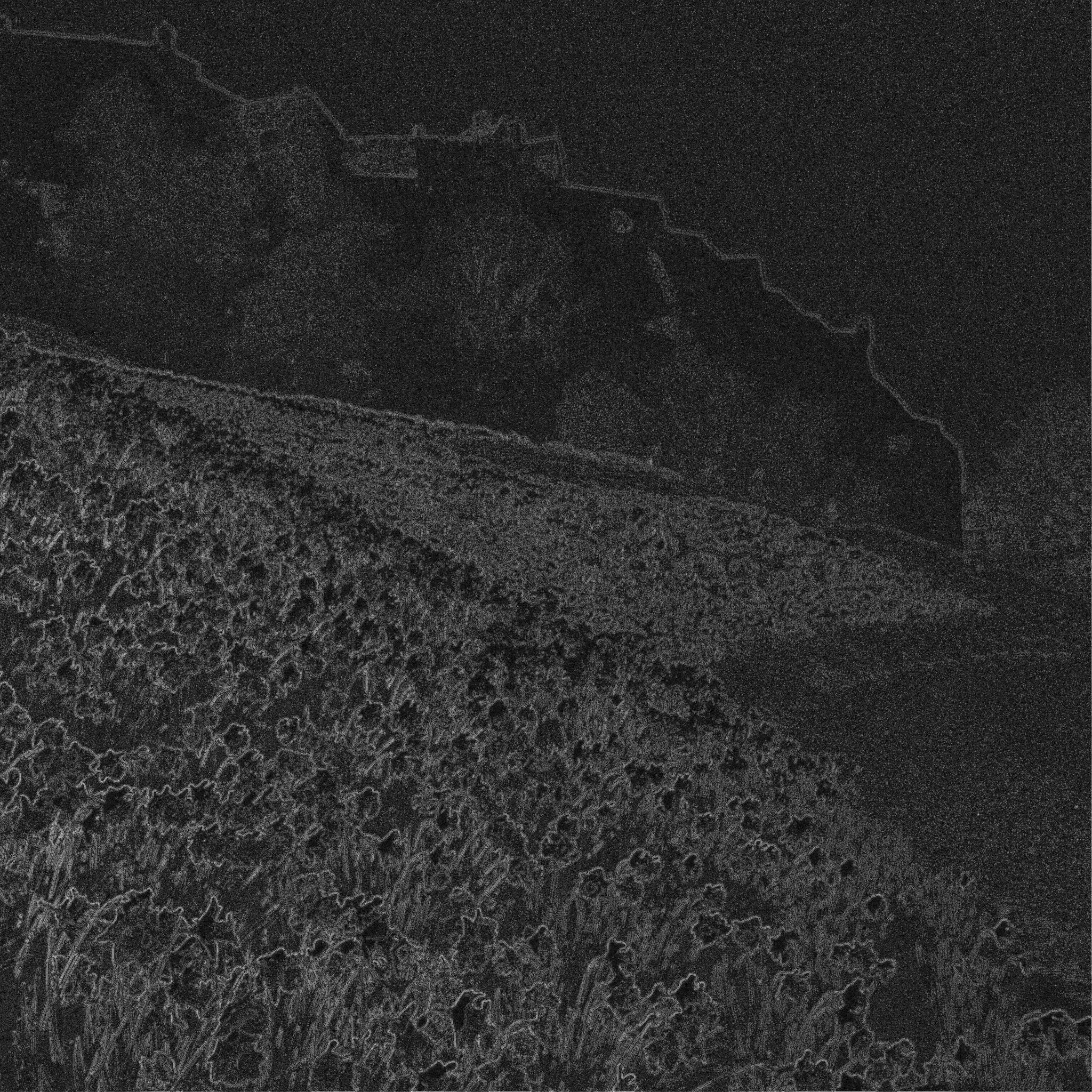
You start with an image that looks like this:

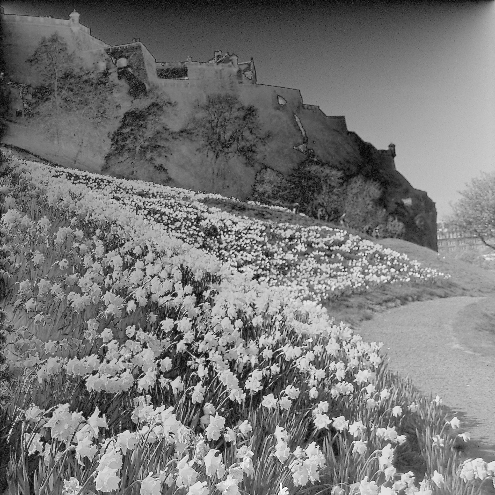
Which has been generated from the original:

First is an image of Edinburgh Castle, processed such that the edges between light and dark areas replace the original picture.

Your job: reconstruct the initial image

This is an artificial thing to do, but it mimics many scientific applications (e.g. that solve systems of PDEs) since the algorithm is iterative, requiring many successive stencil operations.

Each pixel of the new image \(M\) is generated based on its neighboring pixel values and the original edge data \(E\) by repeatedly performing the following update:

\[ M_{i,j} = \frac{M_{i-1,j} + M_{i+1,j} + M_{i,j-1} + M_{i,j+1} - E_{i,j}}{4} \]

The more iterations, the better the reconstruction (although for simplicity we work in greyscale rather than colour).

Run the original

You are provided with a working but slow CUDA implementation of the reconstruction algorithm.

First of all, let’s compile and run the code. The code is set up to run the algorithm on both the GPU and the CPU. It compares the outputs from the two runs to verify correctness, and then displays timings for each run.

Build with make

Choose to work with either C or Fortran

C:

cd src_c
module load nvidia/nvhpc/22.11
make

Fortran:

cd src_fortran
module load nvidia/nvhpc/22.11
make

Run on the batch system

To run, you need to know your budget code. To do this, you need to know your budget code - you can check by logging into SAFEm navigating to the relevant Cirrus login account and checking which budgets it can access.

Submit the job with:

sbatch --account <YOUR BUDGET CODE> submit.sh

Query SLURM for your jobs:

squeue -u $USER

During on campus tutorials we have reserved one node (4 GPUs) for the use of the class. You can access this by editing the SLURM script or adding extra options to the sbatch command:

sbatch --account d171 --qos=reservation
--reservation=<reservation ID>

View the resulting image

On Cirrus you can either:

1. View directly with display if you have set up X11 forwarding when you connected

module load ImageMagick
display output.pgm

2. Use convert to turn the output file into e.g. a jpg or png file and then copy it to your client

module load ImageMagick
convert output.pgm output.jpg

Hopefully you can see that the picture is starting to become clearer. As the algorithm is iterative, there is a loop in the main routine that invokes the kernel \(N=100\) times.

Increasing N will increase the quality of the reconstruction, but please don’t do this during the lab!

If you were to run for 10 million iterations, the resulting image would look like this:

Important note!

Keep a note of the run times of your jobs and what you have changed each time!

Now it’s time to optimise the code and improve on the GPU timing printed when you ran the code, by editing the source code.

Note that a one pixel wide halo region of zeroes is added to each edge of the various image-data arrays; this simplifies the computation as it allows the edge pixels to be treated in the same manner as other pixels.

Note: The edge array, which holds the original edge data, does not have require a halo.

Profiling

You can (should?) profile your code as you optimise it. There are basic submission scripts for both Nsight Systems (profile-nsys.sh) and Compute (profile-ncomp.sh) included. Once you have run these, you can transfer the files to your workstation and analyse them with the GUIs (available from NVIDIA https://developer.nvidia.com/tools-overview).

Minimizing Data Transfer

A challenge with GPUs and other accelerators is that transferring data between host memory and device memory is often relatively slow. An important optimization technique involves minimise the amount of data that is transferred between host and device.

Notice that in the main loop in reconstruct.cu (C) or reconstruct.cuf (Fortran), the data is copied from GPU memory to host memory and then back to GPU memory at each iteration. This is not in fact necessary; with the exception of the final iteration when the data must be copied back to the host, it is going to be processed on the GPU again in the next iteration. Therefore, we can optimise manipulating the GPU memory directly without expensive transfers.

We can simply copy the output array directly to the input array after each iteration.

In order to do this you will need to:

C

• Remove the cudaMemcpy calls from inside the main loop

• Replace them with a cudaMemcpy call to copy, directly on the device, from d_output to d_input

• Add a new cudaMemcpy call after the end of the loop (in between the two calls to get_current_time()) to copy the final result back from the GPU to the output buffer in host memory.

Fortran

• Remove the assignments to output (from d_output) and to d_input (from output), inside the main loop

• Replace them with an assignment directly from d_output to d_input

• Add a new assignment after the end of the loop (in between the two calls to cpu_time()) to copy the final result back from the GPU to the output buffer in host memory

Once you have made these changes, compile and run the code again as above and take note of the time taken by the GPU version.

How does it compare to the previous timing?

Reminder

The GPU performs best when consecutive CUDA threads access consecutive memory locations, allowing memory coalescing.

C

For the kernel in reconstruct_kernels.cu, it can be seen that consecutive threads correspond to consecutive rows of the image, but consecutive memory locations instead correspond to consecutive columns. The threads are not reading from consecutive locations.

Fortran

For the kernel in reconstruct_kernels.cuf, it can be seen that consecutive threads correspond to consecutive columns of the image, but consecutive memory locations instead correspond to consecutive rows. The threads are not reading from consecutive locations.

What to do

• Update the kernel such that the role of the image row and column is reversed, in relation to how pixels are assigned to CUDA threads.

• Since the image is perfectly square, you will not need to change the way the kernel is launched.

• How does the performance compare to the previous version?

GPU codes typically run best when there are many threads running in parallel, each doing a small part of the work. We can achieve this with our image processing code by using a thread for each pixel of the image, rather than for each row or column as before. CUDA supports 1-, 2- or 3-dimensional decompositions. A 2D decomposition maps most naturally onto the pixels of an image.

• Update your both your kernel, and the code responsible for specifying the decomposition such that that a 2D decomposition is over both rows and columns.

• The original code uses 256 threads per block in a 1D CUDA decomposition. Replace this with 16 threads in each of the X and Y directions of the 2D CUDA decomposition, to give a total of 256 threads per block. Ensure that the number of blocks is specified appropriately in each direction.

• Ensure that you retain memory coalescing!

Measure performance and compare to the previous versions.

Once you have the 2D kernel working correctly, you can try altering certain parameters and see what effect this has on its performance. In particular, you can investigate the effects of different grid and block sizes.

How does changing the grid and block sizes affect the total runtime?